3.8: The Many Worlds Interpretation

We conclude this chapter by discussing a set of compelling but controversial ideas arising from the phenomenon of quantum entanglement: the Many Worlds Interpretation as formulated by Hugh Everett (1956).

So far, when describing the phenomenon of state collapse, we have relied on the measurement postulate (see Section 3.2), which is part of the Copenhagen Interpretation of quantum mechanics. This is how quantum mechanics is typically taught, and how physicists think about the theory when doing practical, everyday calculations.

However, the measurement postulate has two bad features:

1. It stands apart from the other postulates of quantum mechanics, for it is the only place where randomness (or “indeterminism”) creeps into quantum theory. The other postulates do not refer to probabilities. In particular, the Schrödinger equation

   \[i\hbar\frac{\partial}{\partial t}|\psi(t)\rangle = \hat{H}(t) |\psi(t)\rangle\]

   is completely deterministic. If you know \(\hat{H}(t)\) and are given the state \(|\psi(t_0)\rangle\) at some time \(t_0\), you can in principle determine \(|\psi(t)\rangle\) for all \(t\). This time-evolution consists of a smooth, non-random rotation of the state vector within its Hilbert space. A measurement process, however, has a completely different character: it causes the state vector to jump discontinuously to a randomly-selected value. It is strange that quantum theory contains two completely different ways for a state to change.

2. The measurement postulate is silent on what constitutes a measurement. Does measurement require a conscious observer? Surely not: as Einstein once exasperatedly asked, are we really expected to believe that the Moon exists only when we look at it? But if a given device interacts with a particle, what determines whether it acts via the Schrödinger equation, or performs a measurement?

The Many Worlds Interpretation seeks to resolve these problems by positing that the measurement postulate is not a fundamental postulate of quantum mechanics. Rather, what we call “measurement”, including state collapse and the apparent randomness of measurement results, is an emergent phenomenon that can be derived from the behavior of complex many-particle quantum systems obeying the Schrödinger equation. The key idea is that a measurement process can be described by applying the Schrödinger equation to a quantum system containing both the thing being measured and the measurement apparatus itself.

We can study this using a toy model formulated by Albrecht (1993). Consider a spin-\(1/2\) particle, and an apparatus designed to measure \(S_z\). Let \(\mathscr{H}_S\) be the spin-\(1/2\) Hilbert space (which is 2D), and \(\mathscr{H}_A\) be the Hilbert space of the apparatus (which has dimension \(d\)). We will assume that \(d\) is very large, as actual experimental apparatuses are macroscopic objects containing \(10^{23}\) or more atoms! The Hilbert space of the combined system is

\[\mathscr{H} = \mathscr{H}_S \otimes \mathscr{H}_A,\]

and is \(2d\)-dimensional. Let us suppose the system is prepared in an initial state

\[|\psi(0)\rangle = \Big(a_+ |\!+z\rangle + a_- |\!-z\rangle\Big) \otimes |\Psi\rangle,\]

where \(a_\pm\in\mathbb{C}\) are the quantum amplitudes for the particle to be initially spin-up or spin-down, and \(|\Psi\rangle \in \mathscr{H}_A\) is the initial state of the apparatus.

The combined system now evolves via the Schrödinger equation. We aim to show that if the Hamiltonian has the form

\[\hat{H} = \hat{S}_z \otimes \hat{V},\]

where \(\hat{S}_z\) is the operator corresponding to the observable \(S_z\), then time evolution has an effect equivalent to the measurement of \(S_z\).

It turns out that we can show this without making any special choices for \(\hat{V}\) or \(|\Psi\rangle\). We only need \(d \gg 2\), and for both \(\hat{V}\) and \(|\Psi\rangle\) to be “sufficiently complicated”. We choose \(|\Psi\rangle\) to be a random state vector, and choose random matrix components for the operator \(\hat{V}\). The precise generation procedures will be elaborated on later. Once we decide on \(|\Psi\rangle\) and \(\hat{V}\), we can evolve the system by solving the Schödinger equation

\[|\psi(t)\rangle = U(t)|\psi(0)\rangle, \;\;\;\mathrm{where}\;\; \hat{U}(t) = \exp\left[-\frac{i}{\hbar}\hat{H}t\right].\]

Because the part of \(\hat{H}\) acting on the \(\mathscr{H}_S\) subspace is \(\hat{S}_z\), the result necessarily has the following form:

\[\begin{align} \begin{aligned}|\psi(t)\rangle &= \hat{U}(t)\Big(a_+ |\!+\!z\rangle + a_- |\!-\!z\rangle\Big) \otimes |\Psi\rangle \\ &= a_+ |\!+\!z\rangle \otimes |\Psi_+(t)\rangle \;+\; a_- |\!-\!z\rangle \otimes |\Psi_-(t)\rangle. \end{aligned}\end{align}\]

Here, \(|\Psi_+(t)\rangle\) and \(|\Psi_-(t)\rangle\) are apparatus states that are “paired up” with the \(|\!+\!z\rangle\) and \(|\!-\!z\rangle\) states of the spin-\(1/2\) subsystem. At \(t=0\), both \(|\Psi_+(t)\rangle\) and \(|\Psi_-(t)\rangle\) are equal to \(|\Psi\rangle\); for \(t > 0\), they rotate into different parts of the state space \(\mathscr{H}_A\). If the dimensionality of \(\mathscr{H}_A\) is sufficiently large, and both \(\hat{V}\) and \(|\Psi\rangle\) are sufficiently complicated, we can guess (and we will verify numerically) that the two state vectors rotate into completely different parts of the state space, so that

\[\langle\Psi_+(t) | \Psi_-(t)\rangle \approx 0 \;\;\;\textrm{for sufficiently large}\;\; t.\]

Once this is the case, the two terms in the above expression for \(|\psi(t)\rangle\) can be interpreted as two decoupled “worlds”. In one world, the spin has a definite value \(+\hbar/2\), and the apparatus is in a state \(|\Psi_+\rangle\) (which might describe, for instance, a macroscopically-sized physical pointer that is pointing to a “\(S_z = +\hbar/2\)” reading). In the other world, the spin has a definite value \(-\hbar/2\), and the apparatus has a different state \(|\Psi_-\rangle\) (which might describe a physical pointer pointing to a “\(S_z = -\hbar/2\)” reading). Importantly, the \(|\Psi_+\rangle\) and \(|\Psi_-\rangle\) states are orthogonal, so they can be rigorously distinguished from each other. The two worlds are “weighted” by \(|a_+|^2\) and \(|a_-|^2\), which correspond to the probabilities of the two possible measurement results.

The above description can be tested numerically. Let us use an arbitrary basis for the apparatus space \(\mathscr{H}_A\); in that basis, let the \(d\) components of the initial apparatus state vector \(|\Psi\rangle\) be random complex numbers:

\[\begin{aligned} \begin{aligned} |\Psi\rangle = \frac{1}{\sqrt{\mathcal{N}}}\, \begin{pmatrix}\Psi_0 \\ \Psi_1 \\ \vdots \\ \Psi_{d-1} \end{pmatrix}, \;\; \mathrm{where} \;\; \mathrm{Re}(\Psi_j), \mathrm{Im}(\Psi_j) \sim N(0,1). \end{aligned}\end{aligned}\]

In other words, the real and imaginary parts of each complex number \(\Psi_j\) are independently drawn from the the standard normal (Gaussian) distribution, denoted by \(N(0,1)\). The normalization constant \(\mathcal{N}\) is defined so that \(\langle\Psi|\Psi\rangle = 1\).

Likewise, we generate the matrix elements of \(\hat{V}\) according to the following random scheme:

\[\begin{align} \begin{aligned}A_{ij} &\sim u_{ij} + i v_{ij}, \;\;\;\mathrm{where}\;\;u_{ij},v_{ij}\sim N(0,1)\\ \hat{V} &= \frac{1}{2\sqrt{d}} \left(\hat{A} + \hat{A}^\dagger\right).\end{aligned}\end{align}\]

This scheme produces a \(d\times d\) matrix with random components, subject to the requirement that the overall matrix be Hermitian. The factor of \(1/2\sqrt{d}\) is relatively unimportant; it ensures that the eigenvalues of \(\hat{V}\) lie in the range \([-2,2]\), instead of scaling with \(d\), see Edelman and Rao (2005).

The Schrödinger equation can now be solved numerically. The results are shown below:

Figure \(\PageIndex{1}\)

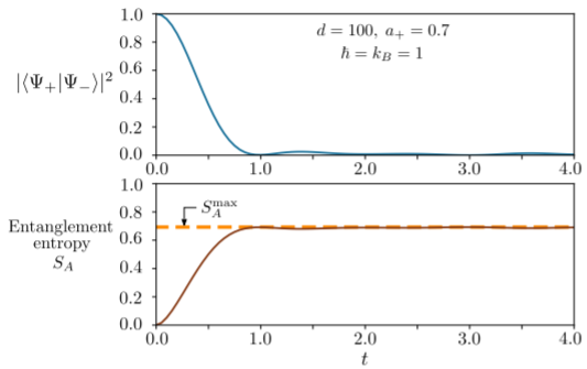
In the initial state, we let \(a_+ = 0.7\), so \(a_- = \sqrt{1-0.7^2} = 0.71414\dots\) The upper panel plots the overlap between the two apparatus states, \(|\langle\Psi_+|\Psi_-\rangle|^2\), versus \(t\). In accordance with the preceding discussion, the overlap is unity at \(t = 0\), but subsequently decreases to nearly zero. For comparison, the lower panel plots the entanglement entropy between the two subsystems, \(S_A = -k_b \mathrm{Tr}_A\left\{\hat{\rho}_A\ln\hat{\rho}_A\right\}\), where \(\hat{\rho}_A\) is the reduced density matrix obtained by tracing over the spin subspace. We find that \(S_A = 0\) at \(t=0\), due to the fact that the spin and apparatus subsystems start out with definite quantum states in \(|\psi(0)\rangle\). As the system evolves, the subsystems become increasingly entangled, and \(S_A\) increases up to

\[S_A^{\mathrm{max}}/k_b = - \Big( |a_+|^2 \ln|a_+|^2 + |a_-|^2\ln|a_-|^2 \Big) \approx 0.693\]

This value is indicated in the figure by a horizontal dashed line, and corresponds to the result of the classical entropy formula for probabilities \(\{|a_+|^2,|a_-|^2\}\). Moreover, we see that the entropy reaches \(S_A^{\mathrm{max}}\) at around the same time that \(|\langle\Psi_+|\Psi_-\rangle|^2\) reaches zero. This demonstrates the close relationship between “measurement” and “entanglement”.

For details about the numerical linear algebra methods used to perform the above calculation, refer to Appendix D.

The “many worlds” concept can be generalized from the above toy model to the universe as a whole. In the viewpoint of the Many Worlds Interpretation of quantum mechanics, the entire universe can be described by a mind-bogglingly complicated quantum state, evolving deterministically according to the Schrödinger equation. This evolution involves repeated “branchings” of the universal quantum state, which continuously produces more and more worlds. The classical world that we appear to inhabit is just one of a vast multitude. It is up to you to decide whether this conception of reality seems reasonable. It is essentially a matter of preference, because the Copenhangen Interpretation and the Many Worlds Interpretation have identical physical consequences, which is why they are referred to as different “interpretations” of quantum mechanics, rather than different theories.