5.2: Dirac's Theory of the Electron

The Dirac Hamiltonian

So far, we have been using $p^2/2m$-type Hamiltonians, which are limited to describing non-relativistic particles. In 1928, Paul Dirac formulated a Hamiltonian that can describe electrons moving close to the speed of light, thus successfully combining quantum theory with special relativity. Another triumph of Dirac’s theory is that it accurately predicts the magnetic moment of the electron.

Dirac’s theory begins from the time-dependent Schrödinger wave equation,

$$i\hbar\, \partial_t\, \psi(\mathbf{r},t) = \hat{H} \psi(\mathbf{r},t). \label{schrod}$$

Note that the left side has a first-order time derivative. On the right, the Hamiltonian $\hat{H}$ contains spatial derivatives in the form of momentum operators. We know that time and space derivatives of wavefunctions are related to energy and momentum by

$$i\hbar\, \partial_t\; \leftrightarrow \; E, \qquad -i\hbar\, \partial_j \;\leftrightarrow \; p_j.$$

We also know that the energy and momentum of a relativistic particle are related by

$$E^2 = m^2c^4 + \sum_{j=1}^3 p_j^2c^2, \label{Erelativistic}$$

where $m$ is the rest mass and $c$ is the speed of light. Note that $E$ and $p$ appear to the same order in this equation. (Following the usual practice in relativity theory, we use Roman indices $j \in \{1,2,3\}$ for the spatial coordinates $\{x,y,z\}$.)

Since the left side of the Schrödinger equation $\eqref{schrod}$ has a first-order time derivative, a relativistic Hamiltonian should involve first-order spatial derivatives. So we make the guess

$$\hat{H} = \alpha_0 mc^2 + \sum_{j=1}^3 \alpha_j \hat{p}_j c, \label{Dirac0}$$

where $\hat{p}_j \equiv -i\hbar \partial/\partial x_j$. The $mc^2$ and $c$ factors are placed for later convenience. We now need to determine the dimensionless “coefficients” $\alpha_0$, $\alpha_1$, $\alpha_2$, and $\alpha_3$.

For a wavefunction with definite momentum $\mathbf{p}$ and energy $E$,

$$\hat{H}\psi = E \psi \;\;\;\Rightarrow \;\;\; \left(\alpha_0mc^2 + \sum_{j=1}^3\alpha_j p_jc\right) \psi = E\,\psi.$$

This is obtained by replacing the $\hat{p}_j$ operators with definite numbers. If $\psi$ is a scalar, this would imply that $\alpha_0 mc^2 + \sum_{j}\alpha_j p_j c = E$ for certain scalar coefficients $\{\alpha_0, \dots, \alpha_3\}$, which does not match the relativistic energy-mass-momentum relation $\eqref{Erelativistic}$.

But we can get things to work if $\psi(\mathbf{r},t)$ is a multi-component wavefunction, rather than a scalar wavefunction, and the $\alpha$’s are matrices acting on those components via the matrix-vector product operation. In that case,

$$\hat{H} = \hat{\alpha}_0 mc^2 + \sum_{j=1}^3 \hat{\alpha}_j \hat{p}_j c, \;\; \mathrm{where}\;\; \hat{p}_j \equiv -i\hbar\, \partial_j, \label{Dirac}$$

where the hats on $\{\hat{\alpha}_0, \dots, \hat{\alpha}_3\}$ indicate that they are matrix-valued. Applying the Hamiltonian twice gives

$$\left(\hat{\alpha}_0mc^2 + \sum_{j=1}^3\hat{\alpha}_j p_j c\right)^{\!2}\; \psi = E^2\,\psi.$$

This can be satisfied if

$$\left(\hat{\alpha}_0 mc^2 + \sum_{j=1}^3\hat{\alpha}_j p_j c\right)^2 = E^2\, \hat{I},$$

where $\hat{I}$ is the identity matrix. Expanding the square (and taking care of the fact that the $\hat{\alpha}_\mu$ matrices need not commute) yields

$$\hat{\alpha}_0^2 m^2c^4 + \sum_j \left(\hat{\alpha}_0 \hat{\alpha}_j + \hat{\alpha}_j \hat{\alpha}_0\right) mc^3 p_j + \sum_{jj'} \hat{\alpha}_j \hat{\alpha}_{j'} \, p_j p_{j'} = E^2\hat{I}.$$

This reduces to Equation $\eqref{Erelativistic}$ if the $\hat{\alpha}_\mu$ matrices satisfy

$$\begin{align} \begin{aligned} \hat{\alpha}_\mu^2 &= \hat{I} \;\;\; \textrm{for} \;\;\mu=0,1,2,3, \;\;\textrm{and} \\ \hat{\alpha}_\mu \hat{\alpha}_\nu + \hat{\alpha}_\nu \hat{\alpha}_\mu &= 0 \;\;\; \textrm{for} \;\;\mu \ne \nu. \end{aligned}\end{align}$$

(We use Greek symbols for indices ranging over the four spacetime coordinates $\{0,1,2,3\}$.) The above can be written more concisely using the anticommutator:

$$\{\hat{\alpha}_\mu, \hat{\alpha}_\nu\} = 2\delta_{\mu\nu}, \;\;\; \textrm{for} \;\;\mu,\nu=0,1,2,3. \label{Dirac_anticomm}$$

Also, we need the $\hat{\alpha}_\mu$ matrices to be Hermitian, so that $\hat{H}$ is Hermitian.

It turns out that the smallest possible Hermitian matrices that can satisfy Equation $\eqref{Dirac_anticomm}$ are $4\times4$ matrices. The choice of matrices (or “representation”) is not uniquely determined. One particularly useful choice is called the Dirac representation:

$$\begin{align} \begin{aligned} \hat{\alpha}_0 &= \begin{bmatrix} \hat{I}\, & \hat{0} \\ \hat{0} & -\hat{I} \end{bmatrix}, \;\;\; \hat{\alpha}_1 = \begin{bmatrix} \hat{0} & \hat{\sigma}_1 \\ \hat{\sigma}_1 & \hat{0} \end{bmatrix} \\ \hat{\alpha}_2 &= \begin{bmatrix} \hat{0} & \hat{\sigma}_2 \\ \hat{\sigma}_2 & \hat{0} \end{bmatrix}, \;\;\; \hat{\alpha}_3 = \begin{bmatrix} \hat{0} & \hat{\sigma}_3 \\ \hat{\sigma}_3 & \hat{0} \end{bmatrix}, \end{aligned} \label{alpha_matrices}\end{align}$$

where $\{\hat{\sigma}_{1}, \hat{\sigma}_{2}, \hat{\sigma}_{3}\}$ denote the usual Pauli matrices. Since the $\hat{\alpha}_\mu$’s are $4\times4$ matrices, it follows that $\psi(\mathbf{r})$ is a four-component field.

Eigenstates of the Dirac Hamiltonian

According to Equation $\eqref{Erelativistic}$, the energy eigenvalues of the Dirac Hamiltonian are

$$E = \pm \sqrt{m^2c^4 + \sum_{j} p_j^2c^2}.$$

This is plotted below:

Figure $\PageIndex{2}$

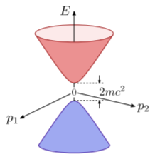
The energy spectrum forms two hyperbolic bands. For each $\mathbf{p}$, there are two degenerate positive energy eigenvalues, and two degenerate negative energy eigenvalues, for a total of four eigenvalues (matching the number of wavefunction components). The upper band matches the dispersion relation for a massive relativistic particle, as desired. But what about the negative-energy band? Who ordered that?

It might be possible for us to ignore the existence of the negative-energy states, if we only ever consider an isolated electron; we could just declare the positive-energy states to be the ones we are interested in, and ignore the others. However, the problem becomes hard to dismiss once we let the electron interact with another system, such as the electromagnetic field. Under such circumstances, the availability of negative-energy states extending down to $E\rightarrow -\infty$ would destabilize the positive-energy electron states, since the electron can repeatedly hop to states with ever more negative energies by shedding energy (e.g., by emitting photons). This is obviously problematic. However, let us wait for a while (till Section 5.2) to discuss how the stability problem might be resolved.

For now, let us take a closer look at the meaning of the Dirac wavefunction. Its four components represent a four-fold “internal” degree of freedom, distinct from the electron’s ordinary kinematic degrees of freedom. Since there are two energy bands, the assignment of an electron to the upper or lower band (or some superposition thereof) consitutes two degrees of freedom. Each band must then posssess a two-fold degree of freedom (so that $2\times 2 = 4$), which turns out to be associated with the electron’s spin.

To see explicitly how this works, let us pick a representation for the $\hat{\alpha}_\mu$ matrices. The choice of representation determines how the four degrees of freedom are encoded in the individual wavefunction components. We will use the Dirac representation $\eqref{alpha_matrices}$. In this case, it is convenient to divide the components into upper and lower parts,

$$\psi(\mathbf{r},t) = \begin{bmatrix}\psi_A(\mathbf{r},t) \\ \psi_B(\mathbf{r},t) \end{bmatrix},$$

where $\psi_A$ and $\psi_B$ have two components each. Then, for an eigenstate with energy $E$ and momentum $\mathbf{p}$, applying $\eqref{alpha_matrices}$ to the Dirac equation $\eqref{Dirac}$ gives

$$\begin{align} \psi_A &= \frac{1}{E - mc^2} \sum_j \hat{\sigma}_j p_j \psi_B, \label{dirac_nonrel1} \\ \psi_B &= \frac{1}{E + mc^2} \sum_j \hat{\sigma}_j p_j \psi_A. \label{dirac_nonrel2}\end{align}$$

Consider the non-relativistic limit, $|\mathbf{p}| \rightarrow 0$, for which $E$ approaches either $mc^2$ or $-mc^2$. For the upper band ($E \gtrsim mc^2$), the vanishing of the denominator in Equation $\eqref{dirac_nonrel1}$ tells us that the wavefunction is dominated by $\psi_A$. Conversely, for the lower band ($E \lesssim -mc^2$), Equation $\eqref{dirac_nonrel2}$ tells us that the wavefunction is dominated by $\psi_B$. We can thus associate the upper ($A$) and lower ($B$) components with the band degree of freedom. Note, however, that this is only an approximate association that holds in the non-relativistic limit! In the relativistic regime, upper-band states can have non-vanishing values in the $B$ components, and vice versa. (There does exist a way to make the upper/lower spinor components correspond rigorously to positive/negative energies, but this requires a more complicated representation than the Dirac representation, for details, see Foldy and Wouthuysen (1950).)

Dirac electrons in an electromagnetic field

To continue pursuing our objective of interpreting the Dirac wavefunction, we must determine how the electron interacts with an electromagnetic field. We introduce electromagnetism by following the same procedure as in the non-relativistic theory (Section 5.1): add $-e\Phi(\mathbf{r},t)$ as a scalar potential function, and add the vector potential via the substitution

$$\hat{\mathbf{p}} \rightarrow \hat{\mathbf{p}} + e\mathbf{A}(\hat{\mathbf{r}},t).$$

Applying this recipe to the Dirac Hamiltonian $\eqref{Dirac}$ yields

$$i\hbar \, \partial_t \psi = \left\{\hat{\alpha}_0 mc^2 -e\Phi(\mathbf{r},t) + \sum_{j} \hat{\alpha}_j \Big[-i\hbar\,\partial_j +eA_j(\mathbf{r},t) \Big] c\right\}\psi(\mathbf{r},t). \label{DiracEM}$$

You can check that this has the same gauge symmetry properties as the non-relativistic theory discussed in Section 5.1.

In the Dirac representation $\eqref{alpha_matrices}$, Equation $\eqref{DiracEM}$ reduces to

$$\begin{align} i\hbar\, \partial_t \, \psi_A &= \big(+mc^2 -e\Phi \big)\, \psi_A \,+\, \sum_{j} \hat{\sigma}_j \big(-i\hbar\partial_j +eA_j \big) \,c\;\psi_B \label{Dirac2a} \\ i\hbar\, \partial_t \, \psi_B &= \big(- mc^2 -e\Phi\big)\, \psi_B \,+\, \sum_{j} \hat{\sigma}_j \big(-i\hbar\partial_j +eA_j \big)\, c\;\psi_A, \label{Dirac2b}\end{align}$$

where $\psi_A$ and $\psi_B$ are the previously-introduced two-component objects corresponding to the upper and lower halves of the Dirac wavefunction.

In the non-relativistic limit, solutions to the above equations can be cast in the form

$$\begin{align} \begin{aligned} \psi_{A}(\mathbf{r},t) &= \Psi_{A}(\mathbf{r},t)\, \exp\left[-i\left(\frac{mc^2}{\hbar}\right)t\right] \\ \psi_{B}(\mathbf{r},t) &= \Psi_{B}(\mathbf{r},t)\, \exp\left[-i\left(\frac{mc^2}{\hbar}\right)t\right]. \end{aligned}\end{align}$$

The exponentials on the right side are the $\exp(-i\omega t)$ factor corresponding to the rest energy $mc^2$, which dominates the electron’s energy in the non-relativistic limit. (Note that by using $+mc^2$ rather than $-mc^2$, we are explicitly referencing the positive-energy band.) If the electron is in an eigenstate with $\mathbf{p} = 0$ and there are no electromagnetic fields, $\Psi_A$ and $\Psi_B$ would just be constants. Now suppose the electron is non-relativistic but not in a $\mathbf{p} = 0$ eigenstate, and the electromagnetic fields are weak but not necessarily vanishing. In that case, $\Psi_A$ and $\Psi_B$ are functions that vary with $t$, but slowly.

Plugging this ansatz into Equations $\eqref{Dirac2a}$–$\eqref{Dirac2b}$ gives

$$\begin{align} i\hbar\, \partial_t \, \Psi_A &= -e\Phi\; \Psi_A \,+\, \sum_{j} \hat{\sigma}_j \big(-i\hbar\partial_j +eA_j \big) c\;\Psi_B \label{Dirac3a} \\ \big(i\hbar\, \partial_t \, + 2mc^2 + e\Phi\big) \Psi_B &= \sum_{j} \hat{\sigma}_j \big(-i\hbar\partial_j +eA_j \big) c\;\Psi_A. \label{Dirac3b}\end{align}$$

On the left side of Equation $\eqref{Dirac3b}$, the $2mc^2$ term dominates over the other two, so

$$\Psi_B \;\approx\; \frac{1}{2mc}\, \sum_{j} \hat{\sigma}_j \big(-i\hbar\partial_j +eA_j \big) \;\Psi_A.$$

Plugging this into Equation $\eqref{Dirac3a}$ yields

$$i\hbar\, \partial_t \, \Psi_A = \left\{-e\Phi \,+\, \frac{1}{2m} \sum_{jk} \hat{\sigma}_j \hat{\sigma}_k \big(-i\hbar\partial_j +eA_j \big) \big(-i\hbar\partial_k +eA_k \big) \right\}\;\Psi_A.$$

Using the identity $\hat{\sigma}_j\hat{\sigma}_k = \delta_{jk}\hat{I} + i \sum_i \varepsilon_{ijk}\sigma_i$:

$$\begin{align} \begin{aligned} i\hbar\, \partial_t \, \Psi_A &= \Bigg\{-e\Phi \,+\, \frac{1}{2m} \big|-i\hbar\nabla +e\mathbf{A} \big|^2 \\ &\qquad+\, \frac{i}{2m} \sum_{ijk} \varepsilon_{ijk} \hat{\sigma}_i \big(-i\hbar\partial_j +eA_j \big) \big(-i\hbar\partial_k +eA_k \big) \Bigg\} \Psi_A. \end{aligned}\end{align}$$

Look carefully at the last term in the curly brackets. Expanding the square yields

$$\frac{i}{2m}\sum_{ijk}\varepsilon_{ijk}\hat{\sigma}_i \Big(-\partial_j\partial_k -i\hbar e \partial_jA_k - i\hbar e \big[A_k\partial_j + A_j\partial_k \big] + e^2A_jA_k \Big).$$

Due to the antisymmetry of $\varepsilon_{ijk}$, all terms inside the parentheses that are symmetric under $j$ and $k$ cancel out when summed over. The only survivor is the second term, which gives

$$\frac{\hbar e}{2m}\sum_{ijk}\varepsilon_{ijk}\hat{\sigma}_i \partial_jA_k = \frac{\hbar e}{2m} \hat{\boldsymbol{\sigma}} \,\cdot\, \mathbf{B}(\mathbf{r},t),$$

where $\mathbf{B} = \nabla\times\mathbf{A}$ is the magnetic field. Hence,

$$i\hbar\, \partial_t \, \Psi_A = \left\{-e\Phi \,+\, \frac{1}{2m} \big|-i\hbar\nabla +e\mathbf{A} \big|^2 \,-\, \left(-\frac{\hbar e}{2m}\, \hat{\boldsymbol{\sigma}}\right) \,\cdot\, \mathbf{B} \right\} \Psi_A.$$

This is an exact match for Equation (5.1.20), except that the Hamiltonian has an additional term of the form $- \hat{\boldsymbol{\mu}} \cdot \hat{\mathbf{B}}$. This additional term corresponds to the potential energy of a magnetic dipole of moment $\boldsymbol{\mu}$ in a magnetic field $\mathbf{B}$. The Dirac theory therefore predicts the electron’s magnetic dipole moment to be

$$|\boldsymbol{\mu}| = \frac{\hbar e}{2m}. \label{Diracmu}$$

Remarkably, this matches the experimentally-observed magnetic dipole moment to about one part in $10^3$. The residual mismatch between Equation $\eqref{Diracmu}$ and the actual magnetic dipole moment of the electron is understood to arise from quantum fluctuations of the electronic and electromagnetic quantum fields. Using the full theory of quantum electrodynamics, that “anomalous magnetic moment” can also be calculated and matches experiment to around one part in $10^9$, making it one of the most precise theoretical predictions in physics! For details, see Zee (2010).

It is noteworthy that we did not set out to include spin in the theory, yet it arose, seemingly unavoidably, as a by-product of formulating a relativistic theory of the electron. This is a manifestation of the general principle that relativistic quantum theory is more constrained than non-relativistic quantum theory Dyson (1951). Due to the demands imposed by relativistic symmetries, spin is not allowed to be an optional part of the theory of the relativistic electron—it has to be built into the theory at a fundamental level.

Positrons and Dirac Field Theory

As noted in Section 5.2, the stability of the quantum states described by the Dirac equation is threatened by the presence of negative-energy solutions. To get around this problem, Dirac suggested that what we regard as the “vacuum” may actually be a state, called the Dirac sea, in which all negative-energy states are occupied. Since electrons are fermions, the Pauli exclusion principle would then forbid decay into the negative-energy states, stabilizing the positive-energy states.

At first blush, the idea seems ridiculous; how can the vacuum contain an infinite number of particles? However, we shall see that the idea becomes more plausible if the Dirac equation is reinterpreted as a single-particle construction which arises from a more fundamental quantum field theory. The Dirac sea idea is an inherently multi-particle concept, and we know from Chapter 4 that quantum field theory is a natural framework for describing multi-particle quantum states. Let us therefore develop this theory.

Consider again the eigenstates of the single-particle Dirac Hamiltonian with definite momenta and energies. Denote the positive-energy wavefunctions by

$$\frac{u_{\mathbf{k}\sigma} \, e^{i\mathbf{k}\cdot \mathbf{r}}}{(2\pi)^{3/2}} = \langle \mathbf{r} | \mathbf{k}, +, \sigma\rangle, \quad\mathrm{where}\;\; \hat{H} |\mathbf{k}, +, \sigma\rangle = \epsilon_{\mathbf{k}\sigma} |\mathbf{k}, +, \sigma\rangle. \label{Diraces1}$$

The negative-energy wavefunctions are

$$\frac{v_{\mathbf{k}\sigma} \, e^{-i\mathbf{k}\cdot \mathbf{r}}}{(2\pi)^{3/2}} = \langle \mathbf{r} | \mathbf{k}, -, \sigma\rangle, \quad\mathrm{where}\;\; \hat{H} |\mathbf{k}, -, \sigma\rangle = - \epsilon_{\mathbf{k}\sigma} |\mathbf{k}, -, \sigma\rangle. \label{Diraces2}$$

Note that $|\mathbf{k}, -, \sigma\rangle$ denotes a negative-energy eigenstate with momentum $-\hbar\mathbf{k}$, not $\hbar\mathbf{k}$. The reason for this notation, which uses different symbols to label the positive-energy and negative-energy states, will become clear later. Each of the $u_{\mathbf{k}\sigma}$ and $v_{\mathbf{k}\sigma}$ terms are four-component objects (spinors), and for any given $\mathbf{k}$, the set

$$\{ u_{\mathbf{k}\sigma}, v_{\mathbf{k},\sigma}\;\; | \;\; \sigma = 1,2 \}$$

forms an orthonormal basis for the four-dimensional spinor space. Thus,

$$\sum_{n} \left(u^n_{\mathbf{k}\sigma}\right)^* u^n_{\mathbf{k}\sigma'} = \delta_{\sigma\sigma'}, \;\; \sum_{n} \left(u^n_{\mathbf{k}\sigma}\right)^* v^n_{\mathbf{k}\sigma'} = 0, \;\; \textrm{etc.} \label{uvorthog}$$

Here we use the notation where $u^n_{\mathbf{k}\sigma}$ is the $n$-th component of the $u_{\mathbf{k}\sigma}$ spinor, and likewise for the $v$’s.

Following the second quantization procedure from Chapter 4, let us introduce a fermionic Fock space $\mathscr{H}_F$, as well as a set of creation/annihilation operators:

$$\begin{align}\begin{aligned} \hat{b}_{\mathbf{k}\sigma}^\dagger \;\; \mathrm{and} \;\; \hat{b}_{\mathbf{k}\sigma} &\;\;\mathrm{create/annihilate} \;\; |\mathbf{k}, +, \sigma\rangle\\ \hat{d}_{\mathbf{k}\sigma}^\dagger \;\; \mathrm{and} \;\; \hat{d}_{\mathbf{k}\sigma} &\;\;\mathrm{create/annihilate} \;\; |\mathbf{k}, -, \sigma\rangle.\end{aligned}\end{align}$$

These obey the fermionic anticommutation relations

$$\begin{align} \begin{aligned} \{\hat{b}_{\mathbf{k}\sigma}, \hat{b}_{\mathbf{k}'\sigma'}^\dagger \} = \delta^3(\mathbf{k}-\mathbf{k}') \, \delta_{\sigma\sigma'}, \quad \{\hat{d}_{\mathbf{k}\sigma}, \hat{d}_{\mathbf{k}'\sigma'}^\dagger \} = \delta^3(\mathbf{k}-\mathbf{k}') \, \delta_{\sigma\sigma'} \\ \{\hat{b}_{\mathbf{k}\sigma}, \hat{b}_{\mathbf{k}'\sigma'} \} = \{\hat{b}_{\mathbf{k}\sigma}, \hat{d}_{\mathbf{k}'\sigma'} \} = \{\hat{d}_{\mathbf{k}\sigma}, \hat{d}_{\mathbf{k}'\sigma'} \} = 0, \;\;\textrm{etc.} \end{aligned} \label{Diracanticommutation0}\end{align}$$

The Hamiltonian is

$$\hat{H} = \int d^3k \sum_\sigma \epsilon_{\mathbf{k}\sigma} \left( \hat{b}^\dagger_{\mathbf{k}\sigma} \hat{b}_{\mathbf{k}\sigma} - \hat{d}^\dagger_{\mathbf{k}\sigma} \hat{d}_{\mathbf{k}\sigma} \right), \label{HDiracQFT0}$$

and applying the annihilation operators to the vacuum state $|\varnothing\rangle$ gives zero:

$$\hat{b}_{\mathbf{k}\sigma} |\varnothing\rangle = \hat{d}_{\mathbf{k}\sigma} |\varnothing\rangle = 0.$$

When formulating bosonic field theory, we defined a local field annihilation operator that annihilates a particle at a given point $\mathbf{r}$. In the infinite-system limit, this took the form

$$\hat{\psi}(\mathbf{r}) = \int d^3k \; \varphi_{\mathbf{k}}(\mathbf{r}) \, \hat{a}_{\mathbf{k}},$$

and the orthonormality of the $\varphi_{\mathbf{k}}$ wavefunctions implied that $[\hat{\psi}(\mathbf{r}), \hat{\psi}^\dagger(\mathbf{r}')] = \delta^3(\mathbf{r}-\mathbf{r}')$. Similarly, we can use the Dirac Hamiltonian’s eigenfunctions $\eqref{Diraces1}$–$\eqref{Diraces2}$ to define

$$\hat{\psi}_n(\mathbf{r}) = \int \frac{d^3k}{(2\pi)^{3/2}} \; \sum_\sigma \left( u^n_{\mathbf{k}\sigma} e^{i\mathbf{k}\cdot\mathbf{r}} \, \hat{b}_{\mathbf{k}\sigma} + v^n_{\mathbf{k}\sigma} e^{-i\mathbf{k}\cdot\mathbf{r}} \, \hat{d}_{\mathbf{k}\sigma}\right). \label{Diracpsi0}$$

Note that there are two terms in the parentheses because the positive-energy and negative-energy states are denoted by differently-labeled annihilation operators. Moreover, since the wavefunctions are four-component spinors, the field operators have a spinor index $n$. Using the spinor orthonormality conditions $\eqref{uvorthog}$ and the anticommutation relations $\eqref{Diracanticommutation0}$, we can show that

$$\left\{\hat{\psi}_n(\mathbf{r}), \hat{\psi}_{n'}^{\dagger}(\mathbf{r}')\right\} = \delta_{nn'}\, \delta^3(\mathbf{r}-\mathbf{r}'),$$

with all other anticommutators vanishing. Hence, $\hat{\psi}_n(\mathbf{r})$ can be regarded as an operator that annihilates a four-component fermion at point $\mathbf{r}$.

Now let us define the operators

$$\hat{c}_{\mathbf{k}\sigma} = \hat{d}^\dagger_{\mathbf{k}\sigma}.$$

Using these, the fermionic anticommutation relations can be re-written as

$$\begin{align} \begin{aligned} \{\hat{b}_{\mathbf{k}\sigma}, \hat{b}_{\mathbf{k}'\sigma'}^\dagger \} = \delta^3(\mathbf{k}-\mathbf{k}') \, \delta_{\sigma\sigma'}, \quad \{\hat{c}_{\mathbf{k}\sigma}, \hat{c}_{\mathbf{k}'\sigma'}^\dagger \} = \delta^3(\mathbf{k}-\mathbf{k}') \, \delta_{\sigma\sigma'} \\ \{\hat{b}_{\mathbf{k}\sigma}, \hat{b}_{\mathbf{k}'\sigma'} \} = \{\hat{b}_{\mathbf{k}\sigma}, \hat{c}_{\mathbf{k}'\sigma'} \} = \{\hat{c}_{\mathbf{k}\sigma}, \hat{c}_{\mathbf{k}'\sigma'} \} = 0, \;\;\textrm{etc.} \end{aligned} \label{Diracanticommutators}\end{align}$$

Hence $\hat{c}^\dagger_{\mathbf{k}\sigma}$ and $\hat{c}_{\mathbf{k}\sigma}$ formally satisfy the criteria to be regarded as creation and annihilation operators. The particle created by $\hat{c}^\dagger_{\mathbf{k}\sigma}$ is called a positron, and is equivalent to the absence of a $d$-type particle (i.e., a negative-energy electron).

The Hamiltonian $\eqref{HDiracQFT0}$ can now be written as

$$\hat{H} = \int d^3k \sum_\sigma \epsilon_{\mathbf{k}\sigma} \left( \hat{b}^\dagger_{\mathbf{k}\sigma} \hat{b}_{\mathbf{k}\sigma} + \hat{c}^\dagger_{\mathbf{k}\sigma} \hat{c}_{\mathbf{k}\sigma} \right) \;\; + \;\; \textrm{constant}, \label{HDiracQFT}$$

which explicitly shows that the positrons have positive energies (i.e., the absence of a negative-energy particle is equivalent to the presence of a positive-energy particle). With further analysis, which we will skip, it can be shown that the positron created by $\hat{c}^\dagger_{\mathbf{k}\sigma}$ has positive charge $e$ and momentum $\hbar\mathbf{k}$. The latter is thanks to the definition adopted in Equation $\eqref{Diraces2}$; the absence of a momentum $-\hbar \mathbf{k}$ particle is equivalent to the presence of a momentum $\hbar \mathbf{k}$ particle. As for the field annihilation operator $\eqref{Diracpsi0}$, it can be written as

$$\hat{\psi}_n(\mathbf{r}) = \int \frac{d^3k}{(2\pi)^{3/2}} \; \sum_\sigma \left( u^n_{\mathbf{k}\sigma} e^{i\mathbf{k}\cdot\mathbf{r}} \, \hat{b}_{\mathbf{k}\sigma} + v^n_{\mathbf{k}\sigma} e^{-i\mathbf{k}\cdot\mathbf{r}} \, \hat{c}^\dagger_{\mathbf{k}\sigma}\right). \label{Diracpsi}$$

The $c$-type annihilation operators do not annihilate $|\varnothing\rangle$. However, let us define

$$|\varnothing'\rangle = \prod_{\mathbf{k}\sigma} \hat{d}_{\mathbf{k}\sigma}^\dagger |\varnothing\rangle,$$

which is evidently a formal description of the Dirac sea state. Then

$$\hat{c}_{\mathbf{k}\sigma} |\varnothing'\rangle = \hat{d}^\dagger_{\mathbf{k}\sigma} \prod_{\mathbf{k}'\sigma'} \hat{d}_{\mathbf{k}'\sigma'}^\dagger |\varnothing\rangle = 0.$$

At the end of the day, we can regard the quantum field theory as being defined in terms of $b$-type and $c$-type operators, using the anticommutators $\eqref{Diracanticommutators}$, the Hamiltonian $\eqref{HDiracQFT}$, and the field operator $\eqref{Diracpsi}$, along with the vacuum state $|\varnothing'\rangle$. The elementary particles in this theory are electrons and positrons with strictly positive energies. The single-particle Dirac theory, with its quirky negative-energy states, can then be interpreted as a special construct that maps the quantum field theory into single-particle language. Even though we actually started from the single-particle description, it is the quantum field theory, and its vacuum state $|\varnothing'\rangle$, that is more fundamental.

There are many more details about the Dirac theory that we will not discuss here. One particularly important issue is how the particles transform under Lorentz boosts and other changes in coordinate system. For such details, the reader is referred to Dyson (1951).