6.3: C- Entropy

“Entropy” is a concept used in multiple fields of science and mathematics to quantify one’s lack of knowledge about a complex system. In physics, its most commonly-encountered form is thermodynamic entropy, which describes the uncertainty about the microscopic configuration, or “microstate”, of a large physical system. In the field of mathematics known as information theory, information entropy (also called Shannon entropy after its inventor C. Shannon) describes the uncertainty about the contents of a transmitted message. One of the most profound developments in theoretical physics in the 20th century was the discovery by E. T. Jaynes that statistical mechanics can be formulated in terms of information theory; hence, the thermodynamics-based and information-based concepts of entropy are one and the same. For details about this connection, see Jaynes (1957) and Jaynes (1957a). This appendix summarizes the definition of entropy in classical physics, and how it is related to other physical quantities.

C.1 Definition

Suppose a system has \(W\) discrete microstates labeled by integers \(\{1,2,3,\dots, W\}\). These microstates are associated with probabilities \(\{p_1, p_2, p_3, \dots, p_W\}\), subject to the conservation of total probability

\[\sum_{i=1}^W p_i = 1.\]

We will discuss how these microstate probabilities are chosen later (see Section 3). Given a set of these probabilities, the entropy is defined as

\[S = - k_b \, \sum_{i=1}^W p_i \ln(p_i). \label{Sdef}\]

Here, \(k_b\) is Boltzmann’s constant, which gives the entropy units of \([E/T]\) (energy per unit temperature); this is a remnant of entropy’s origins in 19th century thermodynamics, and is omitted by mathematicians.

It is probably not immediately obvious why Equation \(\eqref{Sdef}\) is useful. To understand it better, consider its behavior under two extreme scenarios:

• Suppose the microstate is definitely known, i.e., \(p_k = 1\) for some \(k\). Then \(S = 0\).
• Suppose there are \(W\) possible microstates, each with equal probabilities

  \[p_i = \frac{1}{W} \;\;\forall i \in \{1,2,\dots,W\}.\]

  This describes a scenario of complete uncertainty between the possible choices. Then

  \[S \,=\, -k_b W \frac{1}{W} \ln(1/W) \;=\; k_b \ln W.\]

The entropy formula is designed so that any other probability distribution—i.e., any situation of partial uncertainty—yields an entropy \(S\) between \(0\) and \(k_b \ln W\).

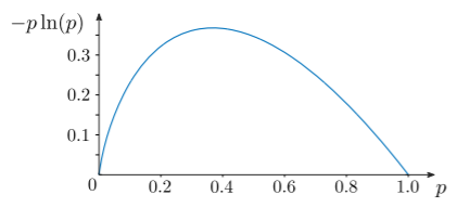
To see that zero is the lower bound for the entropy, note that for \(0 \le p_i \le 1\), each term in the entropy formula \(\eqref{Sdef}\) satisfies \(-k_b\, p_i\ln(p_i) \ge 0\), and the equality holds if and only if \(p_i = 0\) or \(p_i = 1\). This is illustrated in the figure below:

Figure \(\PageIndex{1}\)

This implies that \(S\ge 0\). Moreover, \(S = 0\) if and only if \(p_i = \delta_{ik}\) for some \(k\) (i.e., there is no uncertainty about which microstate the system is in).

Next, it can be shown that \(S\) is bounded above by \(k_b \ln W\), a relation known as Gibbs’ inequality. This follows from the fact that \(\ln x \le x - 1\) for all positive \(x\), with the equality occurring if and only if \(x = 1\). Take \(x = 1/(Wp_i)\) where \(W\) is the number of microstates:

\[\begin{align} \begin{aligned} \ln \left[\frac{1}{Wp_i}\right] &\le \frac{1}{Wp_i} - 1 \quad \textrm{for}\;\textrm{all}\; i = 1,\dots, W. \\ \sum_{i=1}^W p_i \ln \left[\frac{1}{Wp_i}\right] &\le \sum_{i=1}^W \left(\frac{1}{W} - p_i\right) \\ - \sum_{i=1}^W p_i \ln W - \sum_{i=1}^W p_i \ln p_i &\le 1 - 1 = 0 \\ - k_b \sum_{i=1}^W p_i \ln p_i &\le k_b \ln W. \end{aligned}\end{align}\]

Moreover, the equality holds if and only if \(p_i = 1/W\) for all \(i\).

C.2 Extensivity

Another important feature of the entropy is that it is extensive, meaning that it scales proportionally with the size of the system. Consider two independent systems \(A\) and \(B\), which have microstate probabilities \(\{p_i^A\}\) and \(\{p_j^B\}\). If we treat the combination of \(A\) and \(B\) as a single system, each microstate of the combined system is specified by one microstate of \(A\) and one of \(B\), with probability \(p_{ij} = p^A_ip^B_j\). The entropy of the combined system is

\[\begin{align} \begin{aligned} S &= - k_b \sum_{ij} p_i^Ap^B_j \ln\left(p^A_ip^B_j\right) \\ &= - k_b \Big(\sum_{i} p^A_i \ln p^A_i\Big)\Big(\sum_j p^B_j\Big) - k_b \Big(\sum_{i} p^A_i \Big) \Big(\sum_j p^B_j \ln p^B_j\Big) \\ &= S_A + S_B, \end{aligned}\end{align}\]

where \(S_A\) and \(S_B\) are the individual entropies of the \(A\) and \(B\) subsystems.

C.3 Entropy and Thermodynamics

The theory of statistical mechanics seeks to describe the macroscopic behavior of a large physical system by assigning some set of probabilities \(\{p_1, p_2, \dots, p_W\}\) to its microstates. How are these probabilities chosen? One elegant way is to use the following postulate:

Postualte \(\PageIndex{1}\)

Choose \(\{p_1, \dots, p_W\}\) so as to maximize \(S\), subject to constraints imposed by known facts about the macroscopic state of the system.

The idea is that we want a probability distribution that is as “neutral” as possible, while being consistent with the available macroscopic information about the system.

For instance, suppose the only information we have about the macroscopic state of the system is that its energy is precisely \(E\). In this scenario, called a micro-canonical ensemble, we maximize \(S\) by assigning equal probability to every microstate of energy \(E\), and zero probability to all other microstates, for reasons discussed in Section 1. (In some other formulations of statistical mechanics, this assignment of equal probabilities is treated as a postulate, called the ergodic hypothesis.)

Or suppose that only the system’s mean energy \(\langle E \rangle\) is known, and nothing else. In this case, we can maximize \(S\) using the method of Lagrange multipliers. The relevant constraints are the given value of \(\langle E \rangle\) and conservation of probability:

\[\langle E \rangle = \sum_i E_i \,p_i, \quad \sum_i p_i = 1.\]

We thus introduce two Lagrange multiplers, \(\lambda_1\) and \(\lambda_2\). For every microstate \(i\), we require

\[\begin{align}\begin{aligned} \frac{\partial S}{\partial p_i} + \lambda_1 \frac{\partial}{\partial p_i} \left(\sum_j E_j p_j\right) + \lambda_2 \frac{\partial}{\partial p_i} \left(\sum_j p_j\right) &= 0 \\ \Rightarrow \quad - k_b \left(\ln p_i + 1\right) + \lambda_1 E_i + \lambda_2 &= 0.\end{aligned}\end{align}\]

Upon taking \(\lambda_1 = - 1/T\) as the definition of the temperature \(T\), we obtain the celebrated Boltzmann distribution:

\[p_i = \frac{e^{-E/k_bT}}{Z}, \;\;\;\mathrm{where}\;\; Z = \sum_i e^{-E/k_b T}.\]

Further Reading

• E. T. Jaynes, Information theory and statistical mechanics, Physical Review 106, 620 (1957).
• E. T. Jaynes, Information theory and statistical mechanics. ii, Physical Review 108, 171 (1957).