
6.2: B- The Transfer Matrix Method


- Last updated
- May 1, 2021
- Save as PDF

( \newcommand{\kernel}{\mathrm{null}\,}\)
The transfer matrix method is a numerical method for solving the 1D Schrödinger equation, and other similar equations. In this method, the wavefunction at each point is decomposed into two complex numbers, called wave components. The wave components at any two points are related by a complex 2×2 matrix, called the transfer matrix.
B.1 Wave Components in 1D
For a 1D space with spatial coordinates x, the Schrödinger wave equation is
−ℏ22md2ψdx2+V(x)ψ(x)=Eψ(x),
where m is the particle mass, ψ(x) is the wavefunction, V(x) is the potential function, and E is the energy. We treat E as an adjustable parameter (e.g., the energy of the incident particle in a scattering experiment).
Within any region of space where V is constant, the Schrödinger equation reduces to a 1D Helmholtz equation, whose general solution is
ψ(x)=Aeikx+Be−ikx,wherek=√2m[E−V(x)]ℏ2.
If E>V, then the wave-number k is real and positive, and exp(±ikx) denotes a right-moving (+) or left-moving (−) wave. If E<V, then k is purely imaginary, and we choose the branch of the square root so that it is a positive multiple of i, so that exp(±ikx) denotes a wave that decreases exponentially toward the right (+) or toward the left (−).
We can re-write the two terms on the right-hand side as
ψ(x)=ψ+(x)+ψ−(x).
At each position x, the complex quantities ψ±(x) are called the wave components .
The problem statement for the transfer matrix method is as follows. Suppose we have a piecewise-constant potential function V(x), which takes on values {V1,V2,V3,…} in different regions of space, as shown in the figure below:

Given the wave components {ψ+(xa),ψ−(xa)} at one position xa, we seek to compute the wave components {ψ+(xb),ψ−(xb)} at another position xb. In general, these are related by a linear relation
Ψb=M(xb,xa)Ψa,
where
Ψb=[ψ+(xb)ψ−(xb)],Ψa=[ψ+(xa)ψ−(xa)].
The 2×2 matrix M(xb,xa) is called a transfer matrix. Take note of the notation in the parentheses: we put the “start point” xa in the right-hand input, and the “end point” xb in the left-hand input. We want to find M(xb,xa) from the potential and the energy E.
B.2 Constructing the Transfer Matrix
Consider the simplest possible case, where the potential has a single constant value V everywhere between two positions xa and xb, with xb>xa. Then, as we have just discussed, the solution throughout this region takes the form
ψ(x)=Aeikx+Be−ikx,wherek=√2m(E−V)ℏ2,
for some A,B∈C. The wave components at the two positions are
Ψa=[AeikxaBeikxa],Ψb=[AeikxbBeikxb].
Each component of Ψb is exp[ik(xb−xa)] times the corresponding component of Ψa. We can therefore eliminate A and B, and write
Ψb=M0(k,xb−xa)Ψa,whereM0(k,L)≡[eikL00e−ikL].
The 2×2 matrix M0(k,L) is the transfer matrix across a segment of constant potential. Its first input is the wave-number within the segment (determined by the energy E and potential V), and its second input is the segment length.
Next, consider a potential step at some position x0, as shown in the figure below:
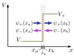
Let xa and xb be two points that are infinitesimally close to the potential step on either side (i.e., xa=x0−0+ and xb=x0+0+, where 0+ denotes a positive infinitesimal). To the left of the step, the potential is V−; to the right, the potential is V+. The corresponding wave-numbers are
k±=√2m(E−V±)ℏ2
There are two important relations between the wavefunctions on the two sides of the step. Firstly, any quantum mechanical wavefunction must be continuous everywhere (otherwise, the Schrödinger equation would not be well-defined); this includes the point x0, so
ψ+(xa)+ψ−(xa)=ψ+(xb)+ψ−(xb).
Secondly, since the potential is non-singular at x0 the derivative of the wavefunction should be continuous at that point (this can be shown formally by integrating the Schrödinger across an infinitesimal interval around x0). Hence,
ik−[ψ+(xa)−ψ−(xa)]=ik+[ψ+(xb)−ψ−(xb)].
These two equations can be combined into a single matrix equation:
[11k−−k−][ψ+(xa)ψ−(xa)]=[11k+−k+][ψ+(xb)ψ−(xb)].
After doing a matrix inversion, this becomes
Ψb=Ms(k+,k−)Ψa,whereMs(k+,k−)=12[1+k−k+1−k−k+1−k−k+1+k−k+].
The 2×2 matrix Ms(k+,k−) is the transfer matrix to go rightward from a region of wave-number k−, to a region of wave-number k+. Note that when k−=k+, this reduces to the identity matrix, as expected.
Using the above results, we can find the transfer matrix for any piecewise-constant potential. Consider the potential function shown below. It consists of segments of length L1,L2,…LN, with potential V1,V2,…,VN; outside, the potential is V0:
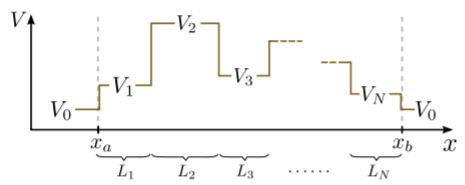
Let xa and xb lie right beyond the first and last segments (where V=V0), with xb>xa. We can compute Ψb by starting with Ψa, and left-multiplying by a sequence of transfer matrices, one after the other. These transfer matrices consist of the two types derived in the previous sections: M0 (to cross a uniform segment) and Ms (to cross a potential step). Each matrix multiplication “transfers” us to another point to the right, until we reach xb.
The overall transfer matrix between the two points is
Definition: Transfer Matrix
M(xb,xa)=Ms(k0,kN)M0(kN,LN)Ms(kN,kN−1)⋯⋯M0(k2,L2)Ms(k2,k1)M0(k1,L1)Ms(k1,k0)whereM0(k,L)=[eikL00e−ikL]Ms(k+,k−)=12[1+k−k+1−k−k+1−k−k+1+k−k+]kn=√2m(E−Vn)ℏ2.
The expression for M(xb,xa) should be read from right to left. Starting from xa, we cross the potential step into segment 1, then pass through segment 1, cross the potential step from segment 1 to segment 2, pass through segment 2, and so forth. (Note that as we move left-to-right through the structure, the matrices are assembled right-to-left; a common mistake when writing a program to implement the transfer matrix method is to assemble the matrices in the wrong order, i.e. right-multiplying instead of left-multiplying.)
B.3 Reflection and Transmission Coefficients
The transfer matrix method is typically used to study how a 1D potential scatters an incident wave. Consider a 1D scatterer that is confined within a region xa≤x≤xb:
V(x)=0forx<xaorx>xb.
The total wavefunction consists of an incident wave and a scattered wave,
ψ(x)=ψi(x)+ψs(x).
The incident wave is assumed to be incident from the left:
ψi(x)=Ψiexp[ik0(x−xa)],wherek0=√2mEℏ2.
We have inserted the extra phase factor of exp(−ik0xa) to ensure that ψi(xa)=Ψi, which will be convenient. The wave is scattered as it meets the structure, and part of it is reflected back to the left, while another part is transmitted across to the right. Due to the linearity of the Schrödinger wave equation, the total wavefunction must be directly proportional to Ψi. Let us write the wave components at xz and xb as
Ψ(xa)=[ψ+(xa)ψ−(xa)]=Ψi[1r]Ψ(xb)=[ψ+(xb)ψ−(xb)]=Ψi[t0].
The complex numbers r and t are called the reflection coefficient and the transmission coefficient, respectively. Their values do not depend on Ψi, since they specify the wave components for the reflected and transmitted waves relative to Ψi. Note also that there is no ψ− wave component at xb, as the scattered wavefunction must be purely outgoing.

From the reflection and transmisison coefficients, we can also define the real quantities
R=|r|2,T=|t|2,
which are called the reflectance and transmittance respectively. These are directly proportional to the total current flowing to the left and right.
According to the transfer matrix relation,
[t0]=M(xb,xa)[1r].
Hence, r and t can be expressed in terms of the components of the transfer matrix:
r=M21M22,t=M11M22−M12M21M22=det