
4.3: Relativistic Momentum
- Page ID
- 3440

\( \newcommand{\vecs}[1]{\overset { \scriptstyle \rightharpoonup} {\mathbf{#1}} } \)
\( \newcommand{\vecd}[1]{\overset{-\!-\!\rightharpoonup}{\vphantom{a}\smash {#1}}} \)
\( \newcommand{\dsum}{\displaystyle\sum\limits} \)
\( \newcommand{\dint}{\displaystyle\int\limits} \)
\( \newcommand{\dlim}{\displaystyle\lim\limits} \)
\( \newcommand{\id}{\mathrm{id}}\) \( \newcommand{\Span}{\mathrm{span}}\)
( \newcommand{\kernel}{\mathrm{null}\,}\) \( \newcommand{\range}{\mathrm{range}\,}\)
\( \newcommand{\RealPart}{\mathrm{Re}}\) \( \newcommand{\ImaginaryPart}{\mathrm{Im}}\)
\( \newcommand{\Argument}{\mathrm{Arg}}\) \( \newcommand{\norm}[1]{\| #1 \|}\)
\( \newcommand{\inner}[2]{\langle #1, #2 \rangle}\)
\( \newcommand{\Span}{\mathrm{span}}\)
\( \newcommand{\id}{\mathrm{id}}\)
\( \newcommand{\Span}{\mathrm{span}}\)
\( \newcommand{\kernel}{\mathrm{null}\,}\)
\( \newcommand{\range}{\mathrm{range}\,}\)
\( \newcommand{\RealPart}{\mathrm{Re}}\)
\( \newcommand{\ImaginaryPart}{\mathrm{Im}}\)
\( \newcommand{\Argument}{\mathrm{Arg}}\)
\( \newcommand{\norm}[1]{\| #1 \|}\)
\( \newcommand{\inner}[2]{\langle #1, #2 \rangle}\)
\( \newcommand{\Span}{\mathrm{span}}\) \( \newcommand{\AA}{\unicode[.8,0]{x212B}}\)
\( \newcommand{\vectorA}[1]{\vec{#1}} % arrow\)
\( \newcommand{\vectorAt}[1]{\vec{\text{#1}}} % arrow\)
\( \newcommand{\vectorB}[1]{\overset { \scriptstyle \rightharpoonup} {\mathbf{#1}} } \)
\( \newcommand{\vectorC}[1]{\textbf{#1}} \)
\( \newcommand{\vectorD}[1]{\overrightarrow{#1}} \)
\( \newcommand{\vectorDt}[1]{\overrightarrow{\text{#1}}} \)
\( \newcommand{\vectE}[1]{\overset{-\!-\!\rightharpoonup}{\vphantom{a}\smash{\mathbf {#1}}}} \)
\( \newcommand{\vecs}[1]{\overset { \scriptstyle \rightharpoonup} {\mathbf{#1}} } \)
\(\newcommand{\longvect}{\overrightarrow}\)
\( \newcommand{\vecd}[1]{\overset{-\!-\!\rightharpoonup}{\vphantom{a}\smash {#1}}} \)
\(\newcommand{\avec}{\mathbf a}\) \(\newcommand{\bvec}{\mathbf b}\) \(\newcommand{\cvec}{\mathbf c}\) \(\newcommand{\dvec}{\mathbf d}\) \(\newcommand{\dtil}{\widetilde{\mathbf d}}\) \(\newcommand{\evec}{\mathbf e}\) \(\newcommand{\fvec}{\mathbf f}\) \(\newcommand{\nvec}{\mathbf n}\) \(\newcommand{\pvec}{\mathbf p}\) \(\newcommand{\qvec}{\mathbf q}\) \(\newcommand{\svec}{\mathbf s}\) \(\newcommand{\tvec}{\mathbf t}\) \(\newcommand{\uvec}{\mathbf u}\) \(\newcommand{\vvec}{\mathbf v}\) \(\newcommand{\wvec}{\mathbf w}\) \(\newcommand{\xvec}{\mathbf x}\) \(\newcommand{\yvec}{\mathbf y}\) \(\newcommand{\zvec}{\mathbf z}\) \(\newcommand{\rvec}{\mathbf r}\) \(\newcommand{\mvec}{\mathbf m}\) \(\newcommand{\zerovec}{\mathbf 0}\) \(\newcommand{\onevec}{\mathbf 1}\) \(\newcommand{\real}{\mathbb R}\) \(\newcommand{\twovec}[2]{\left[\begin{array}{r}#1 \\ #2 \end{array}\right]}\) \(\newcommand{\ctwovec}[2]{\left[\begin{array}{c}#1 \\ #2 \end{array}\right]}\) \(\newcommand{\threevec}[3]{\left[\begin{array}{r}#1 \\ #2 \\ #3 \end{array}\right]}\) \(\newcommand{\cthreevec}[3]{\left[\begin{array}{c}#1 \\ #2 \\ #3 \end{array}\right]}\) \(\newcommand{\fourvec}[4]{\left[\begin{array}{r}#1 \\ #2 \\ #3 \\ #4 \end{array}\right]}\) \(\newcommand{\cfourvec}[4]{\left[\begin{array}{c}#1 \\ #2 \\ #3 \\ #4 \end{array}\right]}\) \(\newcommand{\fivevec}[5]{\left[\begin{array}{r}#1 \\ #2 \\ #3 \\ #4 \\ #5 \\ \end{array}\right]}\) \(\newcommand{\cfivevec}[5]{\left[\begin{array}{c}#1 \\ #2 \\ #3 \\ #4 \\ #5 \\ \end{array}\right]}\) \(\newcommand{\mattwo}[4]{\left[\begin{array}{rr}#1 \amp #2 \\ #3 \amp #4 \\ \end{array}\right]}\) \(\newcommand{\laspan}[1]{\text{Span}\{#1\}}\) \(\newcommand{\bcal}{\cal B}\) \(\newcommand{\ccal}{\cal C}\) \(\newcommand{\scal}{\cal S}\) \(\newcommand{\wcal}{\cal W}\) \(\newcommand{\ecal}{\cal E}\) \(\newcommand{\coords}[2]{\left\{#1\right\}_{#2}}\) \(\newcommand{\gray}[1]{\color{gray}{#1}}\) \(\newcommand{\lgray}[1]{\color{lightgray}{#1}}\) \(\newcommand{\rank}{\operatorname{rank}}\) \(\newcommand{\row}{\text{Row}}\) \(\newcommand{\col}{\text{Col}}\) \(\renewcommand{\row}{\text{Row}}\) \(\newcommand{\nul}{\text{Nul}}\) \(\newcommand{\var}{\text{Var}}\) \(\newcommand{\corr}{\text{corr}}\) \(\newcommand{\len}[1]{\left|#1\right|}\) \(\newcommand{\bbar}{\overline{\bvec}}\) \(\newcommand{\bhat}{\widehat{\bvec}}\) \(\newcommand{\bperp}{\bvec^\perp}\) \(\newcommand{\xhat}{\widehat{\xvec}}\) \(\newcommand{\vhat}{\widehat{\vvec}}\) \(\newcommand{\uhat}{\widehat{\uvec}}\) \(\newcommand{\what}{\widehat{\wvec}}\) \(\newcommand{\Sighat}{\widehat{\Sigma}}\) \(\newcommand{\lt}{<}\) \(\newcommand{\gt}{>}\) \(\newcommand{\amp}{&}\) \(\definecolor{fillinmathshade}{gray}{0.9}\)Learning Objectives
- Explain relativity and momentum
- Global conservation of momentum
The Energy-Momentum Vector
Newtonian mechanics has two different measures of motion, kinetic energy and momentum, and the relationship between them is nonlinear, e.g., doubling your car’s momentum quadruples its kinetic energy. However, nonrelativistic mechanics cannot handle massless particles, which are always ultrarelativistic. We saw in Section 4.1 that ultrarelativistic particles are “generic,” in the sense that they have no individual mechanical properties other than an energy and a direction of motion. Therefore the relationship between kinetic energy and momentum must be linear for ultrarelativistic particles. For example, doubling the amplitude of an electromagnetic wave quadruples both its energy density, which depends on \(E^2\) and \(B^2\), and its momentum density, which goes like \(E×B\).
How can we make sense of these energy-momentum relationships, which seem to take on two completely different forms in the limiting cases of very low and very high velocities?
The first step is realize that since mass and energy are equivalent, we will get more of an apples-to-apples comparison if we stop talking about a material object’s kinetic energy and consider instead its total energy E, which includes a contribution from its mass.
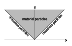
Figure \(\PageIndex{1}\) is a graph of energy versus momentum. In this representation, massless particles, which have \(E \propto |p|\), lie on two diagonal lines that connect at the origin. If we like, we can pick units such that the slopes of these lines are plus and minus one. Material particles lie above these lines. For example, a car sitting in a parking lot has \(p = 0\) and \(E = m\).
Now what happens to such a graph when we change to a different frame or reference that is in motion relative to the original frame? A massless particle still has to act like a massless particle, so the diagonals are simply stretched or contracted along their own lengths. A transformation that always takes a line to a line is a linear transformation, and if the transformation between different frames of reference preserves the linearity of the lines \(p = E\) and \(p = -E\), then it’s natural to suspect that it is actually some kind of linear transformation. In fact the transformation must be linear, because conservation of energy and momentum involve addition, and we need these laws to be valid in all frames of reference. But now by the same reasoning as in section 1.3, the transformation must be area-preserving. We then have the same three cases to consider as in figure 1.1.10. The “Galilean” version is ruled out because it would imply that particles keep the same energy when we change frames. (This is what would happen if \(c\) were infinite, so that the mass-equivalent \(E/c^2\) of a given energy was zero, and therefore \(E\) would be interpreted purely as the mass.) Nor can the “rotational” version be right, because it doesn’t preserve the \(E = |p|\) diagonals. We are left with the third case, which establishes the following aesthetically appealing fact:
Energy-momentum is a four-vector
Let an isolated object have momentum and mass-energy \(p\) and \(E\). Then the \(p-E\) plane transforms according to exactly the same kind of Lorentz transformation as the \(x-t\) plane. That is, \((E,p_x,p_y,p_z)\) is a four-dimensional vector just like \((t,x,y,z)\).
This is a highly desirable result. If it were not true, it would be like having to learn different mathematical rules for different kinds of three-vectors in Newtonian mechanics.
The only remaining issue to settle is whether the choice of units that gives invariant \(45\)-degree diagonals in the \(x-t\) plane is the same as the choice of units that gives such diagonals in the \(p-E\) plane. That is, we need to establish that the \(c\) that applies to \(x\) and \(t\) is equal to the \(c'\) needed for \(p\) and \(E\), i.e., that the velocity scales of the two graphs are matched up. This is true because in the Newtonian limit, the total mass-energy \(E\) is essentially just the particle’s mass, and then \(p/E \approx p/m \approx v\). This establishes that the velocity scales are matched at small velocities, which implies that they coincide for all velocities, since a large velocity, even one approaching \(c\), can be built up from many small increments. (This also establishes that the exponent \(n\) defined section 4.1 equals \(1\) as claimed.)
Suppose that a particle is at rest. Then it has \(p = 0\) and mass energy \(E\) equal to its mass \(m\). Therefore the inner product of its \((E,p)\) four-vector with itself equals \(m^2\). In other words, the “magnitude” of the energy-momentum four-vector is simply equal to the particle’s mass. If we transform into a different frame of reference, in which \(p \neq 0\), the inner product stays the same. In symbols,
\[m^2 = E^2 - p^2\]
or, in units with \(c \neq 1\),
\[(mc^2)^2 = E^2 - (pc)^2\]
We take this as the relativistic definition of mass. Since the definition is an inner product, which is a scalar, it is the same in all frames of reference. (Some older books use an obsolete convention of referring to mγ as “mass” and m as “rest mass.”)
Exercise \(\PageIndex{1}\)
Interpret the equation m^2 = E^2 −p^2 in the case where \(m = 0\).
A high-precision test of this fundamental relativistic relationship was carried out by Meyer et al. in 1963 by studying the motion of electrons in static electric and magnetic fields. They define the quantity
\[Y^2 = \frac{E^2}{m^2 + p^2}\]
which according to special relativity should equal \(1\). Their results, tabulated in the sidebar, show excellent agreement with theory.
Example \(\PageIndex{1}\): Mass of two light waves
Let the momentum of a certain light wave be \((p_t,p_x) = (E,E)\), and let another such wave have momentum \((E,-E)\). The total momentum is \((2E,0)\). Thus this pair of massless particles has a collective mass of \(2E\). This is an example of the non-additivity of relativistic mass.
Collision Invariants
Example \(\PageIndex{1}\) shows that mass is not additive, nor it is a measure of the “quantity of matter.” More generally, suppose that we have a collision between two objects, which could be two cars or two nuclei in a particle accelerator. Conservation of (spatial) momentum dictates that not all the energy is available for smashing windshields or creating gamma rays. For example, a Martian watching a parking lot fender-bender through a powerful telescope would say that both cars were going as fast as fighter jets, due to the rotation of the earth, but this doesn’t make the bang any louder. To avoid being misled by these frame-dependent distractions, we can concentrate only on quantities that are scalars. For a two-body collision, there are three such scalars that we can construct: \(P_{1}^{2}\), \(P_{2}^{2}\), and \(P_1 \cdot P_2\). (The notation \(a^2\) is simply an abbreviation for \(a \cdot a\).) These are known as the collision invariants. The first two of these are simply the squared masses of the individual particles.
Now consider the center of mass frame, i.e., the frame in which the total momentum has a zero spacelike part. In this frame, the total energy-momentum vector is of the form \((E_{cm},0)\), corresponding to a mass \(M = E_{cm}\). All of this energy is available to make a bang. If we were colliding particles in an accelerator in order to produce new particles, this collision would be just barely enough energy to create a single particle of mass \(M\), if the two incoming particles were annihilated in the process. This center of mass energy can be expressed in terms of the collision invariants as
\[\begin{align} M^2 &= (P_1 + P_2)^2 + P_{1}^{2} + P_{2}^{2} + 2P_1 \cdot P_2 \\[5pt] &= m_{1}^{2} + m_{2}^{2} + 2P_1 \cdot P_2 \end{align}\]
This is a nonlinear relationship, and the third collision invariant \(P_1 \cdot P_2\) tells us how the nonlinearity plays out based on the relative directions of motion. The two momentum vectors are both timelike and future-directed, so by the reversed triangle equality (section 1.5) we have
\[M \geq m_1 + m_2\]
Some examples involving momentum
Example \(\PageIndex{2}\): Finding velocity given energy and momentum
If we know that a particle has mass-energy \(E\) and momentum \(p\) (which also implies knowledge of its mass m),what is its velocity?
Solution
In the particle’s rest frame it has a world-line that points straight up on a spacetime diagram, and its momentum vector \(p\) likewise points up in the \(p-E\) plane. Since displacement vectors and momentum vectors transform according to the same rules, this parallelism will be maintained in other frames as well. Therefore in an arbitrarily chosen frame, the vector \(p = (E,p)\) lies along a line whose inverse slope \(v = p/E\) gives the velocity.
As a check on our result, we look at its limiting behavior. In the Newtonian limit, the mass-energy \(E\) is nearly all due to the mass, so we have \(v \approx p/m\), the Newtonian result. In the opposite limit of ultrarelativistic motion, with \(E \gg m\), the definition of mass \(m^2 = E^2 - p^2\) gives \(E \approx |p|\), and we have \(|v| \approx 1\), which is also correct.
Example \(\PageIndex{3}\): Light rays don’t interact
We observe that when two rays of light crosspaths, they continue through one another without bouncing like material objects. This behavior follows directly from conservation of energy-momentum.
Any two vectors can be contained in a single plane, so we can choose our coordinates so that both rays have vanishing \(p_z\). By choosing the state of motion of our coordinate system appropriately, we can also make \(p_y = 0\), so that the collision takes place along a single line parallel to the \(x\)-axis. Since only \(p_x\) is nonzero, we write it simply as \(p\). In the resulting \(p-E\) plane, there are two possibilities: either the rays both lie along the same diagonal, or they lie along different diagonals. If they lie along the same diagonal, then there cannot be a collision, because the two rays are both moving in the same direction at the same speed \(c\), and the trailing one will never catch up with the leading one.
Now suppose they lie along different diagonals. We add their energy-momentum vectors to get their total energy-momentum, which will lie in the gray area of figure \(\PageIndex{1}\). That is, a pair of light rays taken as a single system act sort of like a material object with a nonzero mass. By a Lorentz transformation, we can always find a frame in which this total energy-momentum vector lies along the \(E\) axis. This is a frame in which the momenta of the two rays cancel, and we have a symmetric head-on collision between two rays of equal energy. It is the “center-of-mass” frame, although neither object has any mass on an individual basis. For convenience, let’s assume that the \(x-y-z\) coordinate system was chosen so that its origin was at rest in this frame.
Since the collision occurs along the \(x\)-axis, by symmetry it is not possible for the rays after the collision to depart from the \(x\)-axis; for if they did, then there would be nothing to determine the orientation of the plane in which they emerged. 1 Therefore we are justified in continuing to use the same \(p_x-E\) plane to analyze the four-vectors of the rays after the collision.
Example \(\PageIndex{4}\): Compton scattering
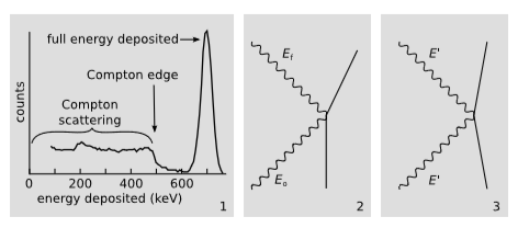
Figure \(\PageIndex{2}\) (1) is a histogram of gamma rays emitted by a \(^{137}\textrm{Cs}\) source and recorded by a NaI scintillation detector. This type of detector, unlike a Geiger-Muller counter, gives a pulse whose height is proportional to the energy of the radiation. About half the gamma rays do what we would like them to do in a detector: they deposit their full energy of \(662\: keV\) in the detector, resulting in a prominent peak in the histogram. The other half, however, interact through a process called Compton scattering, in which they collide with one of the electrons but emerge from the collision still retaining some of their energy, with which they may escape from the detector. The amount of energy deposited in the detector depends solely on the billiard-ball kinematics of the collision, and can be determined from conservation of energy-momentum based on the scattering angle. Forward scattering at \(0\) degrees is no interaction at all, and deposits no energy, while scattering at \(180\) degrees deposits the maximum energy possible if the only interaction inside the detector is a single Compton scattering. We will analyze the \(180\)-degree scattering, since it can be tackled in \(1+1\) dimensions.
Figure \(\PageIndex{2}\) (2) shows the collision in the lab frame, where the electron is initially at rest. As is conventional in this type of diagram, the world-line of the photon is shown as a wiggly line; the wiggles are just a decoration, and the actual world-line consists of two line segments. The photon enters the detector with the full energy \(E_o = 662\: keV\) and leaves with a smaller energy \(E_f\). The difference \(E_o - E_f\) is what the detector will measure, contributing a count to the Compton edge. In the lab frame, the total initial momentum vector is \(p = (E_o + m,E_o)\), with the timelike component representing the total mass-energy. Because the photon is massless, its momentum \(p_x = E_o\) is equal to its energy.
Let \(v\) be the velocity of the center-of-mass frame, \(e/3\), relative to the lab frame. Using the result of example \(\PageIndex{2}\), we find
\[v = \frac{E_o}{E_o + m}\]
To make the writing easier we define
\[\alpha = E_o/m\]
so that
\[v = \frac{\alpha }{1 + \alpha }\]
The transformation from the lab frame to the c.m. frame Doppler shifts the energy of the incident photon down to
\[E' = D(-v)E_o\]
The collision reverses the spatial part of the photon’s energy-momentum vector while leaving its energy the same. Transformation back into the lab frame gives
\[E_f = D(-v)E' = D(-v)^2E_o = \frac{E_o}{1 + 2\alpha }\]
(This can also be rewritten using the quantum mechanical relation \(E = hc/λ\) to give the compact form \(λ_f - λ_o = 2hc/m\).) The final result for the energy of the Compton edge is
\[E_o - E_f = \frac{E_o}{1 + \tfrac{1}{2\alpha }}\]
in good agreement with figure \(\PageIndex{2}\).
Example \(\PageIndex{5}\): Pair production requires matter
Example 4.2.1 discussed the annihilation of an electron and a positron into two gamma rays, which is an example of turning matter into pure energy. An opposite example is pair production, a process in which a gamma ray disappears, and its energy goes into creating an electron and a positron.
Pair production cannot happen in a vacuum. For example, gamma rays from distant black holes can travel through empty space for thousands of years before being detected on earth, and they don’t turn into electron-positron pairs before they can get here. Pair production can only happen in the presence of matter. When lead is used as shielding against gamma rays, one of the ways the gamma rays can be stopped in the lead is by undergoing pair production.
To see why pair production is forbidden in a vacuum, consider the process in the frame of reference in which the electron-positron pair has zero total momentum. In this frame, the gamma ray would have to have had zero momentum, but a gamma ray with zero momentum must have zero energy as well. This means that conservation of the momentum vector has been violated: the timelike component of the momentum is the mass-energy, and it has increased from \(0\) in the initial state to atleast \(2mc^2\) in the final state.
Massless particles travel at \(c\)
Massless particles always travel at \(c(= 1)\). For suppose that a massless particle had \(|v| < 1\) in the frame of some observer. Then some other observer could be at rest relative to the particle. In such a frame, the particle’s momentum \(p\) is zero by symmetry, since there is no preferred direction for it. Then \(E^2 = p^2 + m^2\) is zero as well, so the particle’s entire energy-momentum vector is zero. But a vector that vanishes in one frame also vanishes in every other frame. That means we’re talking about a particle that cannot undergo scattering, emission, or absorption, and is therefore undetectable by any experiment. This is physically unacceptable because we don’t consider phenomena (e.g., invisible fairies) to be of physical interest if they are undetectable even in principle.
What about the case of a material particle, i.e., one having mass? Since we already have an equation \(E = mγ\) for the energy of a material particle in terms of its velocity, we can find a similar equation for the momentum,
\[\begin{align} p &= \sqrt{E^2 - m^2} \nonumber \\[5pt] &= m\sqrt{\gamma ^2 - 1} \nonumber \\[5pt] &= m\sqrt{\frac{1}{1 - v^2} - 1} \nonumber \\[5pt] &= m\gamma v \label{rel momentum} \end{align}\]
(a relation that is useful in its own right, and has been verified experimentally, Figure \(\PageIndex{3}\)).
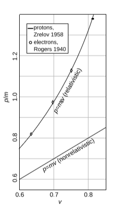
As a material particle gets closer and closer to \(c\), its momentum approaches infinity, so that an infinite force would be required in order to reach \(c\).
In summary, massless particles always move at \(v = c\), while massive ones always move at \(v < c\).
Note that the equation \(p = mγv\) (Equation \ref{rel momentum}) isn’t general enough to serve as a definition of momentum, since it becomes an indeterminate form in the limit \(m \rightarrow 0\).
Example \(\PageIndex{6}\): No half-life for massless particles
Example \(\PageIndex{7}\): Constraints on polarization
We observe that electromagnetic waves are always polarized transversely, never longitudinally. Such a constraint can only apply to a wave that propagates at \(c\). If it applied to a wave that propagated at less than \(c\), we could move into a frame of reference in which the wave was at rest. In this frame, all directions in space would be equivalent, and there would be no way to decide which directions of polarization should be permitted.
Evidence as to which particles are massless
Which of the fundamental particles are massless, and which are not? This is can only be determined empirically, and we have at least one example, the neutrino, that was formerly thought to be massless but is now believed to be massive. For more about the neutrino, see section 4.7. In the present section we discuss bounds on the masses of the photon and the graviton.5 We omit a discussion of the gluon, which would be complicated by the fact that the gluon is never observed as a free particle or as a classical field. This section can be skipped without loss of continuity.
Some readers may exclaim at this point that of course photons must be massless, because light has to travel at the speed of light. But it should be clear from the foregoing presentation that the \(c\) in relativity is not to be interpreted as the speed of light, but as a kind of conversion factor between space and time. If photons have a small but nonvanishing mass, relativity does not have a stake driven through its heart.
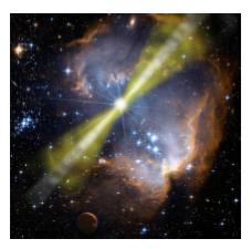
If we want to test whether the photon is massless, the most straightforward technique would seem to be to measure its time of flight as it travels some distance, and see if it goes slower than \(c\). There is a difficulty here because our methods for measuring large distances, e.g., GPS, generally assume that light travels at \(c\). However, if the photon has some mass, then its velocity should depend on its energy, so we can instead test whether the speed of a photon depends on its energy. From quantum mechanics, this is related to its frequency by \(E = hf\), so we are essentially testing whether the speed of light in a vacuum depends on frequency. Presently the best experimental tests of the invariance of the speed of light with respect to wavelength come from astronomical observations of gamma-ray bursts, which are sudden outpourings of high-energy photons, believed to originate from a supernova explosion in another galaxy. One such observation, in 2009,6 collected photons from such a burst, with a duration of \(2\) seconds, indicating that the propagation time of all the photons differed by no more than \(2\) seconds out of a total time in flight on the order of ten billion years, or about one part in \(10^{17}\)!
It turns out, however, that the limits on the mass of the photon imposed by time of flight measurements can be improved on by many orders of magnitude using other methods. In the standard model of particle physics, forces are transmitted by the exchange of particles. We’ll concentrate here on static forces. An electrostatic force is transmitted by the exchange of photons, and a static gravitational force by the exchange of gravitons. Gravity is not part of the standard model of particle physics, and individual gravitons cannot be directly detected by any foreseeable technology,7 but there are fundamental reasons for believing that they must exist, and in any case our discussion is mathematically identical for gravity and electromagnetism. We will therefore discuss electromagnetic fields and then note the corresponding results for gravity.
If we imagine the field surrounding a stationary point charge as a swarm of photons, then the first question that occurs to us is what is the source of the energy needed in order to create them. The standard hand-waving argument is as follows. In addition to the usual momentum-energy form of the Heisenberg uncertainty principle \(\Delta p \Delta x \overset{> }{\sim } h\), there is an energy-time form \(\Delta E \Delta t \overset{> }{\sim } h\). This looks obvious by analogy when we consider that relativistically, energy and momentum are different parts of the energy-momentum four-vector, and likewise for time and position. We can interpret this to mean that it is possible, for short periods of time, to cheat the law of conservation of energy. We can steal a little energy but then pay it back immediately, as long as the duration of the loan is no more than about \(t \sim h/E\). During this time, a virtual particle can travel a distance of no more than \(\sim hc/E\). Now for a massless particle, this energy can be as small as desired, so the force can reach to arbitrarily large distances. But for a massive particle, we have the relativistic relation \(E^2 - p^2 = m^2\), which requires \(E ≥ m\), or \(E ≥ mc^2\) in SI units. This minimum energy corresponds to a maximum range \(\sim h/mc\). In general, we expect that the field carried by a massive particle will fall off more quickly with distance than the field of a massless particle, and we expect that this fall-off will be parametrized somehow by a length scale \(h/mc\).
How would we expect this to play out in the classical theory of electromagnetic fields?
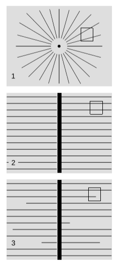
Consider a point charge, figure \(\PageIndex{5}\) (1). Its field lines are straight, and they spread out in all directions, so by observations of any region of space, we can trace the lines backward to see where they would have intersected. That is how far it is from our region of space to the charge. This is a kind of parallax measurement. In the case of gravity, this is exactly what Eratosthenes did in order to measure the radius of the earth.
But now let’s consider the case of an infinite, plane capacitor plate with some charge on it, figure \(\PageIndex{5}\) (2). The field lines don’t spread, so the parallax method doesn’t work. If we examine the field in some small region of space, there should be no way to determine the distance to the capacitor plate. If we believe in Gauss’s law, then the solution is simple: the field is constant in both magnitude and direction, so although it tells us the direction of the nearest point on the plate, it tells us nothing about the distance to that point.
But if the photon is massive, we expect fields to fall off more rapidly with distance than they would according to standard theory. In this example, the standard theory says that the field does not decrease at all with distance, so for a massive photon we expect that it does fall off. This will violate Gauss’s law, but we still expect that the distance to the plate will not be determinable by examination of a small region of space: if the field equations are linear, then a field with a given strength could be from a nearby capacitor plate with a small charge density, or a more distant one with more charge.
If we’re willing to violate Gauss’s law, then we can have field lines simply terminate in empty space, figure \(\PageIndex{1}\) (3), and this will cause the field strength to decrease. As we traverse a small distance \(dx\), moving away from the plate, some fraction of the field lines should terminate, leading to a corresponding fractional reduction \(dE/E\) in the field strength. The ratio \(\frac{\tfrac{dE}{E}}{dx}\) must be constant, and this can only happen if we have \(E \propto e^{-\mu x}\), where \(µ\) is a constant with units of inverse length. (On the other side of the plate, where \(x\) is negative, we have \(+µx\) inside the exponential.) For the reasons discussed above, we actually expect that \(µ\) equals \(mc/h\) multiplied by a unitless constant of order unity. In fact, it can be shown that the unitless constant is a factor of \(2π\), so \(µ\) simply the mass, expressed in units where both \(c\) and \(\hbar\) equal \(1\).
Since the field of a capacitor plate is equal to the superposition of the fields of all the charges distributed uniformly on it, our result that the capacitor’s field falls off in a certain way tells us something corresponding about the field of a point charge. We expect that the field of a point charge \(q\) is
\[E = kq\frac{e^{-\mu r}}{r^2}\]
where Coulomb’s law is recovered in the case \(µ = 0\). This form was originally inferred by Yukawa for nuclear forces, which really do have a finite range.
We now have an extraordinarily sensitive way of placing a limit on the masses of the photon and graviton. Even if \(µ\) is very small, we can make observations on very large distance scales, and static forces should fall off exponentially. In the case of gravitational forces, we observe that gravity does operate, with no detectable Yukawastyle attenuation, on scales comparable to the size of the observable universe, on the order of billions of light-years. This corresponds to a limit on the mass of the graviton of \(\sim 10^{-69}\: kg\)— surely the smallest mass scale that has ever been probed by human beings! Measurements of the magnetic field of Jupiter by the Pioneer 10 space probe limit the mass of the photon to no more than about \(8×10{-52}\: kg\), which is almost as impressive.
Although today’s tightest bounds are from solar-system and cosmological measurements, historically some very precise tabletop experiments were carried out. Laboratory experiments are always desirable in such cases because the conditions can be controlled, and the experiments can be replicated.
No global conservation of energy-momentum in general relativity
If you read chapter 2, you know that the distinction between special and general relativity is defined by the flatness of spacetime, and that flatness is in turn defined by the path independence of parallel transport. Whereas energy is a scalar in Newtonian mechanics, in relativity it is the timelike component of a vector. It therefore follows that in general relativity we should not expect to have global conservation of energy. For a conservation law is a statement that when we add up a certain quantity, the total has a constant value. But if spacetime is curved, then there is no natural, uniquely defined way to compare vectors that are defined at different places in spacetime. We could parallel transport one over to the other, but the result would depend on the path along which we chose to transport it. For similar reasons, we should not expect global conservation of momentum.
This is the answer to a frequently asked question about cosmology. Since 1998 we’ve known that the expansion of the universe is accelerating, rather than decelerating as we would have expected due to gravitational attraction. What is the source of the ever-increasing kinetic energy of all those galaxies? The question assumes that energy must be conserved on cosmological scales, but that just isn’t so.
Nevertheless, general relativity reduces to special relativity on scales small enough to make curvature effects negligible. Therefore it is still valid to expect conservation of energy and momentum to hold locally, as assumed, e.g., in the analysis of Compton scattering in example \(\PageIndex{4}\), and verified in countless experiments.
References
1 In quantum mechanics, there is a loophole here. Quantum mechanics allows certain kinds of randomness, so that the symmetry can be broken by letting the outgoing rays be observed in a plane with some random orientation.
2 There is a second loophole here, which is that a ray of light is actually a wave, and a wave has other properties besides energy and momentum. It has a wavelength, and some waves also have a property called polarization. As a mechanical analogy for polarization, consider a rope stretched taut. Side-to-side vibrations can propagate along the rope, and these vibrations can occur in any plane that coincides with the rope. The orientation of this plane is referred to as the polarization of the wave. Returning to the case of the colliding light rays, it is possible to have nontrivial collisions in the sense that the rays could affect one another’s wavelengths and polarizations. Although this doesn’t actually happen with non-quantum-mechanical light waves, it can happen with other types of waves; see, e.g., Hu et al., arxiv.org/abs/hep-ph/9502276, figure 2. The title of example 4.3.3 is only valid if a “ray” is taken to be something that lacks wave structure. The wave nature of light is not evident in everyday life from observations with apparatus such as flashlights, mirrors, and eyeglasses, so we expect the result to hold under those circumstances, and it does. E.g., flashlight beams do pass through one anther without interacting.
3 See Fiore and Modanese, arxiv.org/abs/hep-th/9508018, and http://physics.stackexchange.com/questions/12488/ decay-of-massless-particles. If such a process does exist, then Lorentz invariance requires that its time-scale be proportional to the particle’s energy. It can be argued that gluons, which are massless, do in fact undergo decay into less energetic gluons, but the interpretation is ambiguous because we never observe gluons as free particles, so we cannot just capture one in a box and watch it rattle around inside until it decays.
4 For an in-depth review of this topic, see Goldhaber and Nieto, “Photon and Graviton Mass Limits,” http://arxiv.org/abs/0809.1003.
5 http://arxiv.org/abs/0908.1832
6 Rothman and Boughn, “Can Gravitons Be Detected?,” http://arxiv.org/ abs/gr-qc/0601043