
1.2: Mixmaster Universe


- Last updated
- Oct 31, 2020
- Save as PDF

( \newcommand{\kernel}{\mathrm{null}\,}\)
Shall we now go on to prove Einstein’s famous mass-energy relationship? May I suggest that you first put on some music to take you elsewhere for a while? If you have not sampled much in the way of 1960s jazz, let me suggest Charles Lloyd’s “Forest Flower” (from the album of the same name, recorded live at the Monterey Jazz Festival in 1966). If you play both the Sunrise and Sunset portions, your brain may then be ready to come on back online.
To prove Einstein’s famous mass-energy relationship most clearly, it helps to return to our graphic calculator from the previous chapter and figure out why it works so well for low-ish speeds.
The Low-velocity Limit
We already know that the time-dilation factor γ is always 1 plus a bit more (actually a lot more at high velocities). Recall the method we used to determine the time dilation for a frame traveling with a velocity v in Figure 1.2.3 of chapter 1. Figure 1.2.1a below uses the same method for v/c = 0.15. In Figure 1.2.1a, the hypotenuse is c t. The length of the vertical side is c τ, and the length of the horizontal side is v t. Let us draw a circle with radius c τ with the upper vertex of the right triangle as the center, as shown in Figure 1.2.1a. Then c t=c τ+f. The relationship between f and γ will be shown later.
The distance f, and its relationship with b, is easiest to see in Figure 1.2.1c, and it’s pretty clear in Figure 1.2.1b, but in Figure 1.2.1a, you really have to squint to see anything. You may simply have to remind yourself that the hypotenuse of a triangle is always longer than either side so there must be a tiny difference between c t and cτ. The tininess of f in Figure 1.2.1a, and its increase as v/c goes from 0.15 to 0.3 to 0.6 in figures 1a through 1c, is the whole point of this discussion.
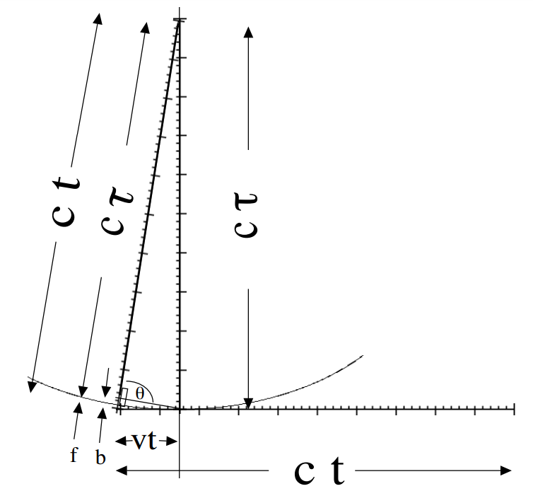
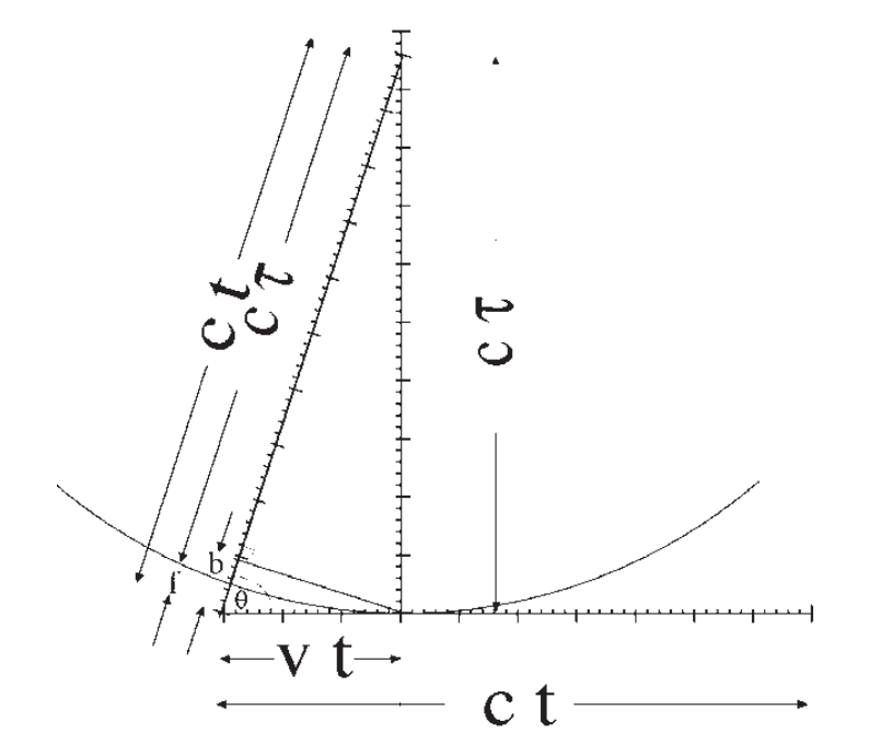
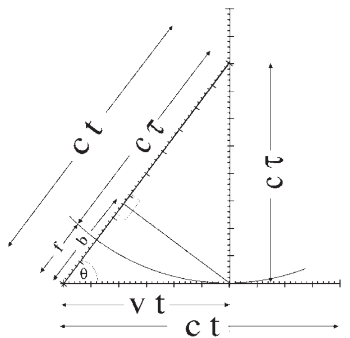
If we overlay the 9.89 cm c τ line in Figure 1.2.1a on the 10 cm hypotenuse c t, the excess is f = 0.11 cm for v c = 0.15. As we double the speed to v c = 0.3, and overlay the 9.54 cm c τ line in Figure 1.2.1b on the 10 cm hypotenuse c t, the excess is f = 0.46 cm. This is a factor of 4.2 times larger than the previous value, or slightly more than the square of 2, the factor by which we increased the velocity. To see if f actually increases with the square of the velocity, let us double it again to v c = 0.6. If we overlay the 8 cm c τ line in Figure 1.2.1c on the 10 cm hypotenuse c t, the excess is f = 2 cm. This is a factor of 4.3 times larger than the previous value, or slightly more than the square of 2—again, the factor by which we increased the velocity. This “slightly more” than the square of 2 also has increased but less quickly as the velocity changed.
We can relate this excess f as the second term on the right-hand side of
γ=tτ≡1√1−v2c2 ,
where the “slightly more” that keeps cropping up is expressed by the factor γ, which we know is “slightly more” than 1. Those willing to put up with several steps of substitutions can look in this footnote* to see the veracity of this relation.
Note
* To see that γ is 1 plus something proportional to v2/c2 plus a slight correction, we can use geometry or the Pythagorean theorem. If you are more comfortable with the latter, skip to the third paragraph of this footnote. Look at figures 1b and 1c, where one can see that I have also drawn in a line perpendicular to the hypotenuse to form a miniature triangle that has exactly the same shape as the triangle with hypotenuse c t, long side c τ, and short side v t, but rotated so that the miniature triangle’s hypotenuse is facing downward. You may remember the term similar triangles from ninth grade geometry: two such triangles have ratios of sides to each other (and, thus, angles) that are the same. The miniature triangle has hypotenuse v t and short side b so the ratios of these two sides for the miniature and big triangle are equal, bvt=vtct or b=v2tc. Finally, we note that the f in figures 1a, 1b, and 1c is in each case about 1/2 b, perhaps with a slight correction unnoticeable to the eye.
Above, when we said we would “overlay the 9.54 cm c τ line in Figure 1.2.1b on the 10 cm hypotenuse c t,” and saw that “the excess is f = 0.46 cm,” we were simply taking the ratio of c t to c τ, which we know is the time-dilation factor γ. Putting these words into ratios,
γ=ctcτ=cτ+fcτ=1+fcτ≅1+12bcτ=1+12v2c2tτ=1+12v2c2γ .
So our guess that f is dependent on the square of the velocity was a good one. If you more or less followed this geometrical method, skip the following.
One could instead use the Pythagorean theorem: We square the hypotenuse ct=cτ+f of the original, big triangle (and expand this square). We then equate it to the sum of the squares of the other two sides:
(f+cτ)2=f2+2fcτ+(cτ)2=(vt)2+(cτ)2.
Since f is small, its square will be much smaller and can be ignored in the above. Canceling the factor of (cτ)2 that appears on both sides and dividing both sides by 2(cτ)2 gives fcτ≅12v2c2tτ, where we have kept one factor of t/τ and set the other one to reproduce the approximation that f is half of b, which gives the fifth version of the equation for γ in the previous paragraph.
Please note that this relation is not an “equation,” since it involves an approximation symbol and has γ, on both the left and right sides. It is an iterative relation that is probably best read as a recipe:
Take a rough value for γ and multiply it by 12v2c2
Add 1 to the result.
Stir for 15 seconds.
Yield: 1 serving of a slightly better version of γ.
We noticed in the last chapter that γ seems to be “1 plus a bit more” for a wide range of velocities. Let us take 1 as our “rough value for γ,” and call it γ0. Our recipe serves up of a slightly better version of γ, which we find to be
γ1≡1+12v2c2γ0=1+12v2c21=1+12v2c2 .
We could keep on going in this fashion and find a third term that will depend on the fourth power of the velocity.
Those of you who are a bit queasy about math can just plug your ears and say “LA LA LA” out loud while I write that one can apply the Pythagorean theorem to Figure 1.2.1 and discover the exact expression for γ to be
γ=tτ≡1√1−v2c2 ,
which involves a square inside a dreaded square root at the bottom of the sea, so it is not as convenient as is our γ1, but you can get numbers out of your calculator for high speeds where our γ1 loses accuracy.* This becomes apparent as we calculate γ1 and γ for various velocities:
| vc | v2c2 | 12v2c2 | γ1≅1+12v2c2 | γ≡1√1−v2c2 |
|---|---|---|---|---|
| 0.1 | 0.01 | 0.005 | 1.005 | 1.00503 |
| 0.2 | 0.04 | 0.02 | 1.02 | 1.02062 |
| 0.3 | 0.09 | 0.045 | 1.045 | 1.04828 |
| 0.4 | 0.16 | 0.08 | 1.08 | 1.09109 |
| 0.5 | 0.25 | 0.125 | 1.125 | 1.15470 |
| 0.6 | 0.36 | 0.18 | 1.18 | 1.25 |
It seems that γ1 works pretty well for velocities below half the speed of light.
Now would be a good time to go put on some obnoxiously loud rock music to release any tension you may have over going through this derivation. May I suggest Led Zeppelin’s The Ocean (Live at Madison Square Garden, 1973)? When you have done that, come on back.
Note
* Did you ever wonder how your calculator actually finds this beast? It uses a series of approximations:
γ=tτ≡(1−v2c2)−12=1−(−12)v2c2+(−12)(−32)2(v2c2)2−⋯
and so on, which confirms that our “‘slightly more’ than [ f ]” above will depend on the fourth power of the velocity and several of higher powers to get 10-digit accuracy.
Into the Mix
Now look closely at figure 8 of chapter 1. The light is reflected from the right-hand mirror at the same time that the light is reflected from the top mirror. These events are simultaneous in the rest frame of the rocket. But in figures 9b and 9c in chapter 1, the light is reflected off the top mirror before it is reflected off the right-hand mirror, not simultaneously! (But the return sequence to the lower left-hand corner is simultaneous for both frames of reference.) The sequence of events in different frames of reference moving relative to each other is not necessarily the same when you live in Einstein’s universe.
The time interval between two events I measure on my clock depends not only on the time interval you measure on your clock (time dilation) but also on where you are standing relative to the other event in your frame of reference. In other words, my time depends on your space too.* In our rocket moving at velocity v=35c, a watch on our astronaut in Figure 1.2.1 of chapter 1 would read a time tw=54τw to us on Earth, while a clock sitting a distance x away on the floor of the spaceship—that our twin asserts is perfectly synchronized with her watch in her frame of reference—would read to us
tc=γτc−xcvc=54τw−35xc ,
but perpendicular distances are unaffected. (For this reason, angles that extend into the x′ direction will be affected.)
Not only does relativity force us to give up “absolute time”; it also forces us to give up the idea that “space” (a three-dimensional world that we can group together as {width, length, and height}—or, if you prefer, {north, west, and up}) and “time” (a one-dimensional marker of {duration}) are entirely separate actualities. We have to begin to perceive the universe as a four-dimensional spacetime. To use a word analogy for the math, a spacetime event that you measure as {duration, width, length, and height} may be perceived by someone else moving relative to you as {duration coupled to length, width, length coupled to duration, and height}.
Just as space and time constitute a four-dimensional entity of the universe {c t, north, west, up}, so do other common quantities like momentum and energy. I had a fairly petite woman named Catherine Wong in my 2013 Freshman Inquiry class who plays rugby (Figure 1.2.2). Suppose you are on the field watching her as she barrels into you heading north. What happens? (You get knocked a few feet north.) What else happens? (Some of her motional energy [kinetic energy, or KE] gets deposited into your body, which you experience as pain in your stomach.) Suppose she instead barrels into you heading west while you were still looking south. What happens? (You get knocked few feet west.) What else? (Some of her KE is deposited into your body, which you experience as pain in your side.) Suppose she instead tosses the ball high above your head and you reach up to catch it. What happens? (Your hands recoil a few inches downward.) What else happens? (Some of the ball’s KE gets deposited into your body, which you experience as stinging palms.)
* x=γ(x−vt) and t=γ(t−vx/c2) for motion in the x direction.

These are each different experiences of our three-dimensional world of momentum that have in common the pain characteristic of the deposition of energy into your body, the final entry in this gang of four, {energy/c, northward momentum, westward momentum, upward momentum}. Just as we usually write the spacetime four-dimensional vector as abbreviated symbols {ct,x,y,z}, so too the energy-momentum four-dimensional vector is written in abbreviated symbols {E/c,px,py,pz}. Why the momentum is px, and not mx, is historical and avoids confusion with the symbol m used for mass.
I do not know Catherine’s weight, so let us just pin it at a nice round number like 100 pounds. Suppose instead of her, a 200-pound player going at the same speed runs into you. How will the pain compare? (It will be worse.) As you might expect, smaller people can often get going much faster than larger people, so imagine now that Catherine is running twice as fast as the 200-pound player. Who is going to hurt you more? That is right, she will. Even if she is only going 50% faster, she will wham you worse and cause more pain. This is a life lesson in respect that is important to learn.
It turns out that a player who runs into you at twice the speed of a second one will hurt you four times as much, but an equal-speed player who is twice as heavy as the first one will hurt you only twice as much. That can be quantified by the relation
KE=12mv2.∗
Exercise 1.2.1
* You can verify that a ball falling 5 meters in 1 second will have a velocity of 10 m/s. Its kinetic energy is equal to the gravitational potential energy it had before falling,
KE=12m(10m/s)2=m(10m/s/s)(5m)=mgh
where g is the acceleration of gravity (10 m/s/s) and h is 5 m
Is Nothing Sacred?
The triangle in Figure 1.2.2 of chapter 1 is a useful way to comprehend a four-dimensional reality on a two-dimensional sheet of paper. The hypotenuse is the time part (c is a constant so c t really just tells us about t), and the horizontal leg, labeled v t, is the space part, since it has to do with the motion of the rocket through space. In special relativity, we can often ignore the fact that space really has three dimensions, because the rocket really only moves along a one-dimensional line.* The third side of the triangle, labeled c τ, represents proper time, an example of a relativistic invariant, something that each of us measures as being the same in our own reference frame. The speed of light c is another example of a relativistic invariant. No matter who measures the half-life of a muon that is at rest relative to their rocket ship, they all get the same value. So although time is relative between moving frames, it is not unknown. We will always agree on what you will measure for t, the lifetime of muons on my rocket, if I am flying past you at velocity v, even though t is not equal to my τ.
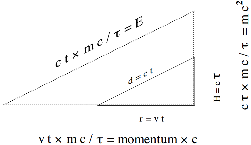
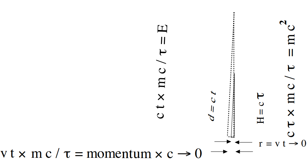
One beautiful element of order in the universe is that it has patterns we can perceive. Suppose we take the triangle in Figure 1.2.2 in chapter 1 and multiply the length of each side by the rocket’s mass (abbreviated as m) and by c and then divide each side of it by proper time τ.†
Then the new figure looks like Figure 1.2.3 below.
* If the rocket starts to curve, it experiences acceleration (like you feel when your car turns a corner), and we must then turn to Einstein’s general theory of relativity, as we do in the next chapter.
† Some readers will have noted that such a procedure is only mathematically valid if mc/τ has the same value in all frames of reference. We know that c is the same in all frames. We defined proper time τ as an invariant quantity, the time interval of two events that occur at the same place (at rest) in any frame of reference. As discussed on page 13, mass m is also an invariant quantity, the same in all frames of reference.
The new triangle has the same shape as the old one. They are called similar triangles, having the same angles between the sides.
Then the hypotenuse of this four-dimensional quantity has length mc2γ≅mc2γ1=mc2+12mv2, where we have approximated γ=t/τ by the first-order approximation γ1 from the first part of this chapter. We see that the second term is precisely the kinetic energy we just defined in the last section, so even though we do not at this point know the meaning of the first term, it must be some kind of energy too, or it would not belong next to the KE term. So we have labeled the hypotenuse as an energy E.
The horizontal leg of the new triangle has the dimensions (units) of the Newtonian momentum (m v) times c, since γ=t/τ is a dimensionless number like 1.25.
The new, stretched vertical leg is a relativistic invariant, mc2.
In the first section of chapter 1, we measured the relative lengths of the sides of the original triangle to get a relationship between times. We now measure the relative lengths of the sides of the new triangle to get a relationship between energies.
If we slow the rocket down so that v is very small, the original triangle is tall and skinny. Since we are stretching each side by the same proportion, keeping the angles the same, the new triangle is also tall and skinny. If we go to the rest frame of the particle, where v = 0, so that the momentum is zero, we find that the hypotenuse, labeled E, is the same length as the vertical leg, labeled mc2. This picture expresses Einstein’s most famous expression,
E0=mc2 ,
where the subscript 0 is a reminder that this expression is only valid for v = 0. This equation (or equivalently, Figure 1.2.4) expresses the revolutionary concept that objects have energy even when they are at rest, called their rest energy.
Another way to say this is that mass and energy are interchangeable. In fact, when we work with particles, we usually express their masses in a unit called an electron volt (eV)— the kinetic energy gained by an electron by “falling” through a one-volt charge difference— divided by the speed of light squared, rather than the kilogram mass unit that is usually used for lumps. Most particles have masses greater than 1 MeV/c2 , where M stands for a million.
The expression E0=mc2 is precisely the source of energy that fuels our Sun, providing the solar energy that warms our bodies and allows our food to grow. A proton, the nucleus of a hydrogen atom, crashes into and sticks to a particle called a deuteron, which has a proton and a neutron bound together. The proton’s mass is 938.7 MeV/c2, and the deuteron’s mass is 1,876.0 MeV/c2. The resulting triton’s mass is 2,809.2 MeV/c2, which is less than the sum of the masses of the proton and deuteron, 2,814.7 MeV/c2. This is OK if the mass difference, 5.5 MeV/c2, is given off as some other form of energy—in this case, a particle of light that is massless and has 5.5 MeV of energy.
Another application of this principle is in particle accelerators that bang two protons together at high speed, converting some of their motional (or kinetic) energy into massive particles, such as the Higgs boson that was in the news in 2014.
The rest energy, like proper time, is a relativistic invariant whose value everyone can measure and agree upon. The general expression for the total energy of a particle is given by the expression E=γE0, just as t=γ τ.* We can use this, for example, in finding the time-dilation factor for the muons created in the Earth’s atmosphere. The muons have an average total energy of 2,000 MeV,† and the mass of a muon is 105 MeV/c2. Then
γ=EE0=Emc2=2000 MeV105 MeV/c2×c2=2000 MeV105 MeV=19,
which is where we got the value we used in the first chapter.
The relativistic relation between a particle’s momentum and energy may be found by taking the ratio of the horizontal leg of Figure 1.2.3 divided by c to the hypotenuse:
pE=mγ vmγ c2=vc2 .
Note that for a particle of light (a photon) whose velocity is v = c, this expression gives a well-defined value of the momentum of a massless particle: p=E/c. You may have read about the spaceship LightSail 2 that demonstrated in 2019 that the sunlight reflecting off its thin Mylar sail transferred its momentum to the spacecraft. One might, thus, use a laser to send a spaceship to Alpha Centauri.
* An alternate but equivalent form is obtainable from Figure 1.2.4 by using the Pythagorean theorem: E2=m2γ2v2c2+m2c4=p2c2+m2c4.
† National Council on Radiation Protection and Measurements, Report No. 94, Exposure of the Population in the United States and Canada from Natural Background Radiation (NCRP, Bethesda, MD, 1987), p. 12.