
1.3: Measurement
- Page ID
- 3419

\( \newcommand{\vecs}[1]{\overset { \scriptstyle \rightharpoonup} {\mathbf{#1}} } \)
\( \newcommand{\vecd}[1]{\overset{-\!-\!\rightharpoonup}{\vphantom{a}\smash {#1}}} \)
\( \newcommand{\dsum}{\displaystyle\sum\limits} \)
\( \newcommand{\dint}{\displaystyle\int\limits} \)
\( \newcommand{\dlim}{\displaystyle\lim\limits} \)
\( \newcommand{\id}{\mathrm{id}}\) \( \newcommand{\Span}{\mathrm{span}}\)
( \newcommand{\kernel}{\mathrm{null}\,}\) \( \newcommand{\range}{\mathrm{range}\,}\)
\( \newcommand{\RealPart}{\mathrm{Re}}\) \( \newcommand{\ImaginaryPart}{\mathrm{Im}}\)
\( \newcommand{\Argument}{\mathrm{Arg}}\) \( \newcommand{\norm}[1]{\| #1 \|}\)
\( \newcommand{\inner}[2]{\langle #1, #2 \rangle}\)
\( \newcommand{\Span}{\mathrm{span}}\)
\( \newcommand{\id}{\mathrm{id}}\)
\( \newcommand{\Span}{\mathrm{span}}\)
\( \newcommand{\kernel}{\mathrm{null}\,}\)
\( \newcommand{\range}{\mathrm{range}\,}\)
\( \newcommand{\RealPart}{\mathrm{Re}}\)
\( \newcommand{\ImaginaryPart}{\mathrm{Im}}\)
\( \newcommand{\Argument}{\mathrm{Arg}}\)
\( \newcommand{\norm}[1]{\| #1 \|}\)
\( \newcommand{\inner}[2]{\langle #1, #2 \rangle}\)
\( \newcommand{\Span}{\mathrm{span}}\) \( \newcommand{\AA}{\unicode[.8,0]{x212B}}\)
\( \newcommand{\vectorA}[1]{\vec{#1}} % arrow\)
\( \newcommand{\vectorAt}[1]{\vec{\text{#1}}} % arrow\)
\( \newcommand{\vectorB}[1]{\overset { \scriptstyle \rightharpoonup} {\mathbf{#1}} } \)
\( \newcommand{\vectorC}[1]{\textbf{#1}} \)
\( \newcommand{\vectorD}[1]{\overrightarrow{#1}} \)
\( \newcommand{\vectorDt}[1]{\overrightarrow{\text{#1}}} \)
\( \newcommand{\vectE}[1]{\overset{-\!-\!\rightharpoonup}{\vphantom{a}\smash{\mathbf {#1}}}} \)
\( \newcommand{\vecs}[1]{\overset { \scriptstyle \rightharpoonup} {\mathbf{#1}} } \)
\(\newcommand{\longvect}{\overrightarrow}\)
\( \newcommand{\vecd}[1]{\overset{-\!-\!\rightharpoonup}{\vphantom{a}\smash {#1}}} \)
\(\newcommand{\avec}{\mathbf a}\) \(\newcommand{\bvec}{\mathbf b}\) \(\newcommand{\cvec}{\mathbf c}\) \(\newcommand{\dvec}{\mathbf d}\) \(\newcommand{\dtil}{\widetilde{\mathbf d}}\) \(\newcommand{\evec}{\mathbf e}\) \(\newcommand{\fvec}{\mathbf f}\) \(\newcommand{\nvec}{\mathbf n}\) \(\newcommand{\pvec}{\mathbf p}\) \(\newcommand{\qvec}{\mathbf q}\) \(\newcommand{\svec}{\mathbf s}\) \(\newcommand{\tvec}{\mathbf t}\) \(\newcommand{\uvec}{\mathbf u}\) \(\newcommand{\vvec}{\mathbf v}\) \(\newcommand{\wvec}{\mathbf w}\) \(\newcommand{\xvec}{\mathbf x}\) \(\newcommand{\yvec}{\mathbf y}\) \(\newcommand{\zvec}{\mathbf z}\) \(\newcommand{\rvec}{\mathbf r}\) \(\newcommand{\mvec}{\mathbf m}\) \(\newcommand{\zerovec}{\mathbf 0}\) \(\newcommand{\onevec}{\mathbf 1}\) \(\newcommand{\real}{\mathbb R}\) \(\newcommand{\twovec}[2]{\left[\begin{array}{r}#1 \\ #2 \end{array}\right]}\) \(\newcommand{\ctwovec}[2]{\left[\begin{array}{c}#1 \\ #2 \end{array}\right]}\) \(\newcommand{\threevec}[3]{\left[\begin{array}{r}#1 \\ #2 \\ #3 \end{array}\right]}\) \(\newcommand{\cthreevec}[3]{\left[\begin{array}{c}#1 \\ #2 \\ #3 \end{array}\right]}\) \(\newcommand{\fourvec}[4]{\left[\begin{array}{r}#1 \\ #2 \\ #3 \\ #4 \end{array}\right]}\) \(\newcommand{\cfourvec}[4]{\left[\begin{array}{c}#1 \\ #2 \\ #3 \\ #4 \end{array}\right]}\) \(\newcommand{\fivevec}[5]{\left[\begin{array}{r}#1 \\ #2 \\ #3 \\ #4 \\ #5 \\ \end{array}\right]}\) \(\newcommand{\cfivevec}[5]{\left[\begin{array}{c}#1 \\ #2 \\ #3 \\ #4 \\ #5 \\ \end{array}\right]}\) \(\newcommand{\mattwo}[4]{\left[\begin{array}{rr}#1 \amp #2 \\ #3 \amp #4 \\ \end{array}\right]}\) \(\newcommand{\laspan}[1]{\text{Span}\{#1\}}\) \(\newcommand{\bcal}{\cal B}\) \(\newcommand{\ccal}{\cal C}\) \(\newcommand{\scal}{\cal S}\) \(\newcommand{\wcal}{\cal W}\) \(\newcommand{\ecal}{\cal E}\) \(\newcommand{\coords}[2]{\left\{#1\right\}_{#2}}\) \(\newcommand{\gray}[1]{\color{gray}{#1}}\) \(\newcommand{\lgray}[1]{\color{lightgray}{#1}}\) \(\newcommand{\rank}{\operatorname{rank}}\) \(\newcommand{\row}{\text{Row}}\) \(\newcommand{\col}{\text{Col}}\) \(\renewcommand{\row}{\text{Row}}\) \(\newcommand{\nul}{\text{Nul}}\) \(\newcommand{\var}{\text{Var}}\) \(\newcommand{\corr}{\text{corr}}\) \(\newcommand{\len}[1]{\left|#1\right|}\) \(\newcommand{\bbar}{\overline{\bvec}}\) \(\newcommand{\bhat}{\widehat{\bvec}}\) \(\newcommand{\bperp}{\bvec^\perp}\) \(\newcommand{\xhat}{\widehat{\xvec}}\) \(\newcommand{\vhat}{\widehat{\vvec}}\) \(\newcommand{\uhat}{\widehat{\uvec}}\) \(\newcommand{\what}{\widehat{\wvec}}\) \(\newcommand{\Sighat}{\widehat{\Sigma}}\) \(\newcommand{\lt}{<}\) \(\newcommand{\gt}{>}\) \(\newcommand{\amp}{&}\) \(\definecolor{fillinmathshade}{gray}{0.9}\)Learning Objectives
- Measurement for relativity
We would like to have a general system of measurement for relativity, but so far we have only an incomplete patchwork. The length of a timelike vector can be defined as the time measured on a clock that moves along the vector. A spacelike vector has a length that is measured on a ruler whose motion is such that in the ruler’s frame of reference, the vector’s endpoints are simultaneous. But there is no third measuring instrument designed for the purpose of measuring lightlike vectors.
Nor do we automagically get a complete system of measurement just by having defined Minkowski coordinates. For example, we don’t yet know how to find the length of a timelike vector such as \((\Delta t,\Delta x) = (2,1)\), and we suspect that it will be not equal \(2\), since the Hafele-Keating experiment tells us that a clock undergoing the motion represented by \(\Delta x = 1\) will probably not agree with a clock carried by the observer whose clock we used in defining these coordinates.
Invariants
The whole topic of measurement is apt to be confusing, because the shifting landscape of relativity makes us feel as if we’ve walked into a Salvador Dali landscape of melting pocket watches. A good way to regain our bearings is to look for quantities that are invariant: they are the same in all frames of reference. A Euclidean invariant, such as a length or an angle, is one that doesn’t change under rotations: all observers agree on its value, regardless of the orientations of their frames of reference. For a relativistic invariant, we require in addition that observers agree no matter what state of motion they have. (A transformation that changes from one inertial frame of reference to another, without any rotation, is called a boost.)
Electric charge is a good example of an invariant. Electrons in atoms typically have velocities of \(0.01\) to \(0.1\) (in our relativistic units, where \(c = 1\)), so if an electron’s charge depended on its motion relative to an observer, atoms would not be electrically neutral. Experiments have been done to test this to the phenomenal precision of one part in \(10^{21}\), with null results.
A vector can never be an invariant, since it changes direction under a rotation. (Some vectors, such as velocities, also change under a boost.) In freshman mechanics, any quantity, such as energy, that wasn’t a vector usually fell into the category we referred to as scalars. In relativity, however, the term “scalar” has a much more restrictive definition, which we’ll discuss in section 6.2.
By the way, beginners in relativity sometimes get confused about invariance as opposed to conservation. They are not the same thing, and neither implies the other. For example, momentum has a direction in space, so it clearly isn’t invariant — but we’ll see in section 4.3 that there is a relativistic version of the momentum vector that is conserved. As in Newtonian mechanics, we don’t care if all observers agree on the momentum of a system — we only care that the law of momentum conservation is valid and has the same form in all frames. Conversely, there are quantities that are invariant but not conserved, mass being an example.
The metric
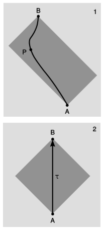
Area in \(1+1\) dimensions is also an invariant, as prove in section 2.5. The invariance of area has little importance on its own, but it provides a good stepping stone toward a relativistic system of measurement. Suppose that we have events \(A\) (Charles VII is restored to the throne) and \(B\) (Joan of Arc is executed). Now imagine that technologically advanced aliens want to be present at both \(A\) and \(B\), but in the interim they wish to fly away in their spaceship, be present at some other event \(P\) (perhaps a news conference at which they give an update on the events taking place on earth), but get back in time for \(B\). Since nothing can go faster than \(c\) (which we take to equal \(1\)), \(P\) cannot be too far away. The set of all possible events \(P\) forms a rectangle, figure \(\PageIndex{1}\), in the \(1+1\)-dimensional plane that has \(A\) and \(B\) at opposite corners and whose edges have slopes equal to \(\pm 1\). We call this type of rectangle a light-rectangle.
The area of this rectangle will be the same regardless of one’s frame of reference. In particular, we could choose a special frame of reference, panel \(2\) of the figure, such that \(A\) and \(B\) occur in the same place. (They do not occur at the same place, for example, in the sun’s frame, because the earth is spinning and going around the sun.) Since the speed \(c = 1\) is the same in all frames of reference, and the sides of the rectangle had slopes \(\pm 1\) in frame \(1\), they must still have slopes \(\pm 1\) in frame \(2\). The rectangle becomes a square, whose diagonals are an \(o\) and an \(s\) for frame \(2\). The length of these diagonals equals the time \(\tau\) elapsed on a clock that is at rest in frame \(2\), i.e., a clock that glides through space at constant velocity from \(A\) to \(B\), reuniting with the planet earth when its orbit brings it to \(B\). The area of the gray regions can be interpreted as half the square of this gliding-clock time, which is called the proper time. “Proper” is used here in the somewhat archaic sense of “own” or “self,” as in “The Vatican does not lie within Italy proper.” Proper time, which we notate \(\tau\), can only be defined for timelike world-lines, since a lightlike or spacelike world-line isn’t possible for a material clock.
In terms of (Minkowski) coordinates, suppose that events \(A\) and \(B\) are separated by a distance \(x\) and a time \(t\). Then in general \(t^2 - x^2\) gives the square of the gliding-clock time.
Proof: Because of the way that area scales with a rescaling of the coordinates, the expression must have the form \((...)t^2+(...)tx+(...)x^2\), where each \((...)\) represents a unitless constant. The \(tx\) coefficient must be zero by the isotropy of space. The \(t^2\) coefficient must equal \(1\) in order to give the right answer in the case of \(x = 0\), where the coordinates are those of an observer at rest relative to the clock. Since the area vanishes for \(x = t\), the \(x^2\) coefficient must equal \(-1\). When \(|x|\) is greater than \(|t|\), events \(A\) and \(B\) are so far apart in space and so close together in time that it would be impossible to have a cause and effect relationship between them, since \(c = 1\) is the maximum speed of cause and effect. In this situation \(t^2 - x^2\) is negative and cannot be interpreted as a clock time, but it can be interpreted as minus the square of the distance between \(A\) and \(B\), as measured in a frame of reference in which \(A\) and \(B\) are simultaneous.
Generalizing to \(3+1\) dimensions and to any vector \(v\), not just a displacement in spacetime, we have a measurement of the vector defined by
\[ v^{2}_{t} - v^{2}_{x} - v^{2}_{y} - v^{2}_{z} \]
In the special case where \(v\) is a spacetime displacement, this can be referred to as the spacetime interval. Except for the signs, this looks very much like the Pythagorean theorem, which is a special case of the vector dot product. We therefore define a function \(g\) called the metric
\[ g( \textbf {u}, \textbf {v}) = u_{t}v_{t} - u_{x}v_{x} - u_{y}v_{y} - u_{z}v_{z} \]
Because of the analogy with the Euclidean dot product, we often use the notation \(u\cdot v\) for this quantity, and we sometimes call it the inner product. The metric is the central object of relativity. In general relativity, which describes gravity as a curvature of spacetime, the coefficients occurring on the right-hand side are no longer \(\pm 1\), but must vary from point to point. Even in special relativity, where the coefficients can be made constant, the definition of \(g\) is arbitrary up to a nonzero multiplicative constant, and in particular many authors define \(g\) as the negative of our definition. The sign convention we use is the most common one in particle physics, while the opposite is more common in classical relativity. The set of signs, \(+---\) or \(-+ ++\), is called the signature of the metric. In section 1.1 we developed the idea of orthogonality of spacetime vectors, with the physical interpretation that if an observer moves along a vector \(o\), a vector s that is orthogonal to \(o\) is a vector of simultaneity. This corresponds to the vanishing of the inner product, \(o\cdot s = 0\), and is only imperfectly analogous to the idea that Euclidean vectors are perpendicular if their dot product is zero. In particular, a nonzero Euclidean vector is never perpendicular to itself, but for any lightlike vector \(v\) we have \(v\cdot v = 0\). The metric doesn’t give us a measure of the length of lightlike vectors. Physically, neither a ruler nor a clock can measure such a vector.
The metric in SI units
Units with \(c = 1\) are known as natural units. (They are natural to relativity in the same sense that units with \(\tilde{h} = 1\) are natural to quantum mechanics.) Any equation expressed in natural units can be reexpressed in SI units by the simple expedient of inserting factors of \(c\) wherever they are needed in order to get units that make sense. The result for the metric could be
\[g( \textbf{u}, \textbf{v}) = c^{2}u_{t}v_{t} - u_{x}v_{x} - u_{y}v_{y} - u_{z}v_{z}\]
or
\[g(\textbf{u},\textbf{v}) = u_{t}v_{t} - (u_{x}v_{x} - u_{y}v_{y} - u_{z}v_{z})/c^{2}\]
It doesn’t matter which we pick, since the metric is arbitrary up to a constant factor. The former expression gives a result in meters, the latter seconds.
Orthogonal light rays?
On a spacetime diagram in \(1+1\) dimensions, we represent the light cone with the two lines \(x = \pm t\), drawn at an angle of \(90\) degrees relative to one another. Are these lines orthogonal? .
No. For example, if \(u = (1,1)\) and \(v = (1,-1)\), then \(u\cdot v\) is \(2\), not zero.
Pioneer 10
The Pioneer 10 space probe was launched in 1972, and in 1973 was the first craft to fly by the planet Jupiter. It crossed the orbit of the planet Neptune in 1983, after which telemetry data were received until 2002. The following table gives the spacecraft’s position relative to the sun at exactly midnight on January 1, 1983 and January 1, 1995. The 1983 date is taken to be \(t = 0\).
| t (s) | x | y | z |
| 0 | 1.784 × 10¹² m | 3.951 × 10¹² m | 0.237 × 10¹² m |
| 3.7869 × 10⁸ s | 2.420 × 10¹² m | 8.827 × 10¹² m | 0.488 × 10¹² m |
Compare the time elapsed on the spacecraft to the time in a frame of reference tied to the sun.
We can convert these data into natural units, with the distance unit being the second (i.e., a light-second, the distance light travels in one second) and the time unit being seconds. Converting and carrying out this subtraction, we have:
| \( \Delta t \) | \( \Delta x \) | \( \Delta y \) | \( \Delta z \) |
| 3.786912 × 10⁸ s | 0.2121 × 10⁴ s | 1.626 × 10⁴ s | 0.084 × 10⁴ s |
Comparing the exponents of the temporal and spatial numbers, we can see that the spacecraft was moving at a velocity on the order of \(10^{-4}\) of the speed of light, so relativistic effects should be small but not completely negligible. Since the interval is timelike, we can take its square root and interpret it as the time elapsed on the spacecraft. The result is \(\tau = 3.786911996×10⁸\, s\). This is \(0.4\, s\) less than the time elapsed in the sun’s frame of reference.
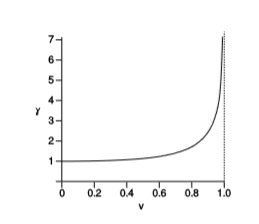
The Gamma Factor
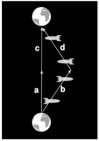
Figure \(\PageIndex{2}\) is the relativistic version of example 1.1.1. We intend to analyze it using the metric, and since the metric gives the same result in any frame, we have chosen for convenience to represent it in the frame in which the earth is at rest. We have \(a = (t,0)\) and \(b = (t,vx)\), where \(v\) is the velocity of the spaceship relative to the earth. Application of the metric gives proper time \(t\) for the earthbound twin and \(t \sqrt{1-v^{2}}\) for the traveling twin. The same results apply for \(c\) and \(d\). The result is that the earthbound twin experiences a time that is greater by a factor \(\gamma\) (Greek letter gamma) defined as \(\gamma = 1/ \sqrt{1-v^{2}}\). If \(v\) is close to \(c\), \(\gamma\) can be large, and we find that when the astronaut twin returns home, still youthful, the earthbound twin can be old and gray. This was at one time referred to as the twin paradox, and it was considered paradoxical either because it seemed to defy common sense or because the traveling twin could argue that she was the one at rest while the earth was moving. The violation of common sense is in fact what was observed in the Hafele-Keating experiment, and the latter argument is fallacious for the same reasons as in the Galilean version given in example 1.1.1.
We have in general the following interpretation:
Time Dilation
A clock runs fastest in the frame of reference of an observer who is at rest relative to the clock. An observer in motion relative to the clock at speed \(v\) perceives the clock as running more slowly by a factor of \(\gamma\).
Although this is phrased in terms of clocks, we interpret it as telling us something about time itself. The attitude is that we should define a concept in terms of the operations required in order to measure it: time is defined as what a clock measures. This philosophy, which has been immensely influential among physicists, is called operationalism and was developed by P.W. Bridgman in the 1920’s. Our operational definition of time works because the rates of all physical processes are affected equally by time dilation. By the time the twins in figure \(\PageIndex{2}\) are reunited, not only has the traveling twin heard fewer ticks from her antique mechanical pocket watch, but she has also had fewer heartbeats, and the ship’s atomic clock agrees with her watch to within the precision of the watch.
Time dilation is symmetrical in the sense that it treats all frames of reference democratically. If observers \(A\) and \(B\) aren’t at rest relative to each other, then \(A\) says \(B’s\) time runs slow, but \(B\) says \(A\) is the slow one. In figure \(\PageIndex{2}\), the laws of physics make no distinction between the frames of reference that coincide with vectors \(a\) and \(b\); as in the corresponding Galilean case of example 1.1.1, the asymmetry comes about because \(a\) and \(c\) are parallel, but \(b\) and \(d\) are not.
As shown in example \(\PageIndex{4}\) below, consistency demands that in addition to the effect on time we have a similar effect on distances:
Length contraction
A meter-stick appears longest to an observer who is at rest relative to it. An observer moving relative to the meter-stick at \(v\) observes the stick to be shortened by a factor of \(\gamma\).
The visualization of length contraction in terms of spacetime diagrams is presented in figure 1.4.3. Our present discussion is limited to \(1+1\) dimensions, but in \(3+1\), only the length along the line of motion is contracted.
An interstellar road trip
Alice stays on earth while her twin Betty heads off in a spaceship for Tau Ceti, a nearby star. Tau Ceti is \(12\) light-years away, so even though Betty travels at \(87\%\) of the speed of light, it will take her a long time to get there: \(14\) years, according to Alice.
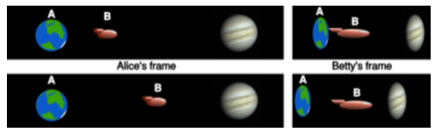
Betty experiences time dilation. At this speed,her \(\gamma\) is \(2.0\), so that the voyage will only seem to her to last \(7\) years. But there is perfect symmetry between Alice’s and Betty’s frames of reference, so Betty agrees with Alice on their relative speed. Betty sees herself as being at rest, while the sun and Tau Ceti both move backward at \(87\%\) of the speed of light. How, then, can she observe Tau Ceti to get to her in only \(7\) years, when it should take \(14\) years to travel \(12\) light-years at this speed?
We need to take into account length contraction. Betty sees the distance between the sun and Tau Ceti to be shrunk by a factor of \(2\). The same thing occurs for Alice, who observes Betty and her spaceship to be foreshortened.
A moving atomic clock
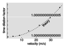
Expanding \(\gamma\) in a Taylor series,we find \(\gamma \approx 1 - v^{2}/2\), so that when \(v\) is small, relativistic effects are approximately proportional to \(v^2\), so it is very difficult to observe them at low speeds. This was the reason that the Hafele-Keating experiment was done aboard passenger jets, which fly at high speeds. Jets, however, fly at high altitude, and this brings in a second time dilation effect, a general-relativistic one due to gravity. The main purpose of the experiment was actually to test this effect. It was not until four decades after Hafele and Keating that anyone did a conceptually simple atomic clock experiment in which the only effect was motion, not gravity. In 2010, however, Chou et al.7 succeeded in building an atomic clock accurate enough to detect time dilation at speeds as low as \(10\, m/s\). Figure \(\PageIndex{5}\) shows their results. Since it was not practical to move the entire clock, the experimenters only moved the aluminum atoms inside the clock that actually made it “tick.”
Large time dilation
The time dilation effects described in example \(\PageIndex{5}\) were very small. If we want to see a large time dilation effect, we can’t do it with something the size of the atomic clocks they used; the kinetic energy would be greater than the total megatonnage of all the world’s nuclear arsenals. We can, however, accelerate subatomic particles to speeds at which \(\gamma\) is large. For experimental particle physicists, relativity is something you do all day before heading home and stopping off at the store for milk. An early,low-precision experiment of this kind was performed by Rossi and Hall in 1941, using naturally occurring cosmic rays. Figure \(\PageIndex{6}\) shows a 1974 experiment of a similar type which verified the time dilation predicted by relativity to a precision of about one part per thousand.
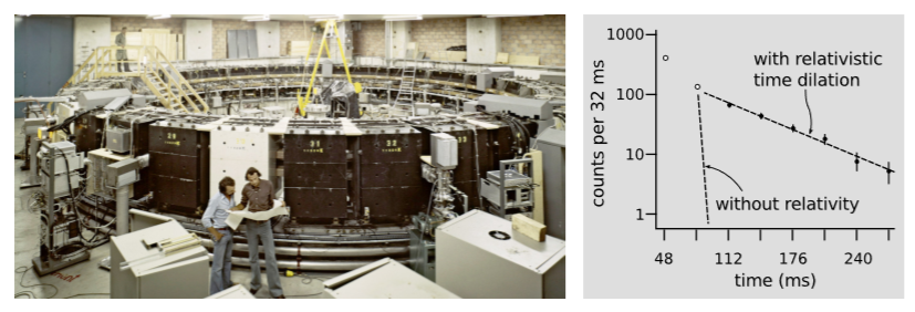
Particles called muons (named after the Greek letter \(\mu\), “myoo”) were produced by an accelerator at CERN, near Geneva. A muon is essentially a heavier version of the electron. Muons undergo radioactive decay, lasting an average of only \(2.197\, µs\) before they evaporate into an electron and two neutrinos. The 1974 experiment was actually built in order to measure the magnetic properties of muons, but it produced a high-precision test of time dilation as a byproduct. Because muons have the same electric charge as electrons, they can be trapped using magnetic fields. Muons were injected into the ring shown in figure \(\PageIndex{6}\), circling around it until they underwent radioactive decay. At the speed at which these muons were traveling, they had \(\gamma = 29.33\), so on the average they lasted \(29.33\) times longer than the normal lifetime. In other words, they were like tiny alarm clocks that self-destructed at a randomly selected time. The graph shows the number of radioactive decays counted, as a function of the time elapsed after a given stream of muons was injected into the storage ring. The two dashed lines show the rates of decay predicted with and without relativity. The relativistic line is the one that agrees with experiment.