1.4: The Lorentz Transformation

Learning Objectives

• Study of the Lorentz transformation

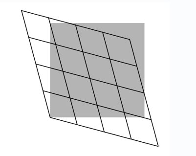
Philosophically, coordinates are unnecessary, but they are convenient. They are arbitrary, so we can change from one set to another. For example, we can change the units used to measure time and position, as in the first and second panels of figure \(\PageIndex{1}\). Nothing changes about the underlying events; only the labels are different. The third panel shows a convenient convention we will use to depict such changes visually. The gray rectangle represents the original grid from the first panel, while the grid of black lines represents the new version from the second panel. Omitting the grid from the gray rectangle makes the diagram easier to decode visually.

Figure \(\PageIndex{1}\): Two events are given as points on a graph of position versus time. Joan of Arc helps to restore Charles VII to the throne. At a later time and a different position, Joan of Arc is sentenced to death.

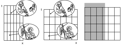
In special relativity it is of interest to convert between the Minkowski coordinates of observers who are in motion relative to one another. The result, shown in figure \(\PageIndex{1}\), is a kind of stretching and smooshing of the diagonals. Since the area is invariant, one diagonal grows by the same factor by which the other shrinks. This change of coordinates is called the Lorentz transformation.

Figure \(\PageIndex{2}\): The Lorentz transformation.

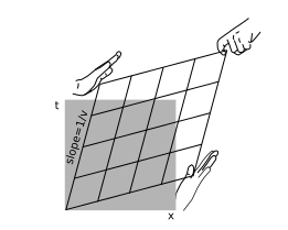
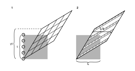
Figure \(\PageIndex{3}\) shows how time dilation and length contraction come about in this picture. It should be emphasized here that the Lorentz transformation includes more effects than just length contraction and time dilation. Many beginners at relativity get confused and come to erroneous conclusions by trying to reduce everything to a matter of inserting factors of \(\gamma\) in various equations. If the Lorentz transformation amounted to nothing more than length contraction and time dilation, it would be merely a change of units like the one shown in figure \(\PageIndex{1}\).

Figure \(\PageIndex{3}\): the figure shows how time dilation and length contraction come about in this picture. It should be emphasized here that the Lorentz transformation includes more effects than just length contraction

The Lorentz transformation can be notated algebraically:

\[t' = \gamma t - \nu\gamma x \\ x' = -\nu\gamma t + \gamma x \label{\(\PageIndex{1}\)}\]

The fact that this is the correct relativistic transformation can be verified by noting that

1. the speed-of-light lines \(x = \pm t\) are preserved, and
2. the determinant equals \(1\).

so that areas are preserved. Alternatively, it is sufficient to check the invariance of the spacetime interval under this transformation.

Equations \(\PageIndex{1}\) treat space and time in a perfectly symmetric way, but this should not be taken as implying that special relativity perfectly embodies such a symmetry. For example, I can easily revisit a place that I’ve been to before, but I can’t go back in time. And of course we have three dimensions of space; our use of \(1+1\) dimensions rather than \(3+1\) is just a matter of convenience for the moment. Note also that there is no exact analogy between figure \(\PageIndex{3}\) (1), where the clock is a pointlike object tracing a line through spacetime, and figure \(\PageIndex{3}\) (2), where the ruler is an extended body that sweeps out a parallel-sided ribbon.

Example \(\PageIndex{1}\): Observers agree on their relative speeds

Observer \(A\) says observer \(B\) is moving away from her at velocity \(v\); is it true, as in Galilean relativity, that \(B\) measures the same speed for \(A\)?

Figure \(\PageIndex{4}\): Obserevers and their relative speeds

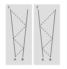
Yes, it is true, but not completely obvious. One way to verify this fact is to check that Lorentz transformations with velocities \(v\) and \(-v\) are inverses. A more physically transparent justification is shown in figure \(\PageIndex{4}\). In figure \(\PageIndex{4}\) (1), \(A\) determines \(B’s\) velocity relative to her by sending out two round-trip signals at the speed of light, and measuring the difference between the two round-trip times. Because space is the same in all directions, the experimental data are exactly the same when \(B\) carries out the measurement, figure \(\PageIndex{4}\) (2), and therefore \(B\) infers the same speed.

Example \(\PageIndex{2}\): Motion in the opposite direction

Figure \(\PageIndex{5}\) shows the case where the observer whose frame is represented by the grid is moving to the left relative to the one whose frame is represented by the gray square.

Figure \(\PageIndex{5}\): Motion in opposite direction

Example \(\PageIndex{3}\): Other quadrants

Figure \(\PageIndex{6}\): Other quadrants

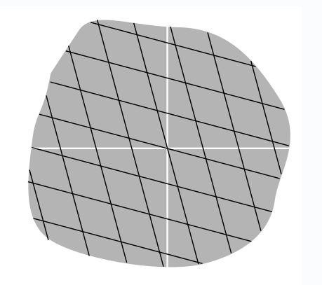
So far I’ve been arbitrarily choosing to draw only the first quad- rant of each coordinate system. Figure \(\PageIndex{6}\) shows a region that includes all four quadrants.

Example \(\PageIndex{4}\): A numerical example of invariance

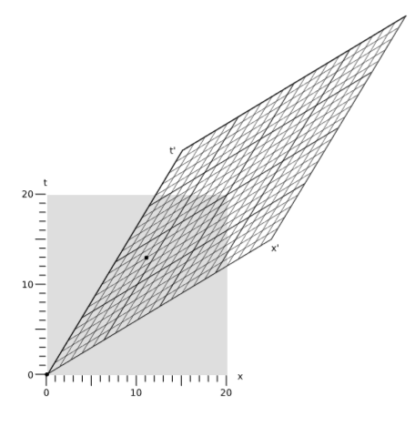
Figure \(\PageIndex{7}\) shows two frames of reference in motion relative to one another at \(v = \frac{3}{5}\). (For this velocity, the stretching and squishing of the main diagonals are both by a factor of \(2\)). Events are marked at coordinates that in the frame represented by the square are

\[(t,x) = (0,0) \\ (t,x) = (13,11)\]

The interval between these events is \(13^2 - 11^2 = 48\). In the frame represented by the parallelogram, the same two events lie at coordinates

\[(t',x') = (0,0) \\ (t',x') = (8,4)\]

Calculating the interval using these values, the result is \(8^2 - 4^2 = 48\), which comes out the same as in the other frame.

Figure \(\PageIndex{7}\): Two frames of reference in motion relative to one another

Example \(\PageIndex{5}\): The garage paradox

One of the most famous of all the so-called relativity paradoxes has to do with our incorrect feeling that simultaneity is well defined. The idea is that one could take a schoolbus and drive it at relativistic speeds into a garage of ordinary size, in which it normally would not fit. Because of the length contraction, the bus would supposedly fit in the garage. The driver, however, will perceive the garage as being contracted and thus even less able to contain the bus.

Figure \(\PageIndex{8}\): In the garage’s frame of reference, the bus is moving, and can fit in the garage due to its length contraction. In the bus’s frame of reference, the garage is moving, and can’t hold the bus due to its length contraction.

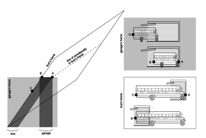
The paradox is resolved when we recognize that the concept of fitting the bus in the garage “all at once” contains a hidden assumption, the assumption that it makes sense to ask whether the front and back of the bus can simultaneously be in the garage. Observers in different frames of reference moving at high relative speeds do not necessarily agree on whether things happen simultaneously. As shown in figure aw. the person in the garage’s frame can shut the door at an instant B he perceives to be simultaneous with the front bumper’s arrival A at the back wall of the garage, but the driver would not agree about the simultaneity of these two events, and would perceive the door as having shut long after she plowed through the back wall.

Example \(\PageIndex{6}\): Shifting clocks

Figure \(\PageIndex{9}\): Shifting clocks

The top row of clocks in the figure \(\PageIndex{9}\) are located in three different places. They have been synchronized in the frame of reference of the earth, represented by the paper. This synchronization is carried out by exchanging light signals (Einstein synchronization). For example, if the front and back clocks both send out flashes of light when they think it’s \(2\) o’clock, the one in the middle will receive them both at the same time. Event \(A\) is the one at which the back clock \(A\) reads \(2\) o’clock, etc.

The bottom row of clocks are aboard the train, and have been synchronized in a similar way. For the reasons discussed in example 1.1.4 in section 1.1, their synchronization differs from that of the earth-based clocks. By referring to the diagram of the Lorentz transformation shown on the right, we see that in the frame of the train, \(2\), \(C\) happens first, then \(B\), then \(A\).

This is an example of the interpretation of the term \(t' = \dots - \nu\gamma x\) in the Lorentz transformation (eq. \(\PageIndex{1}\)). Because the events occur at different \(x’s\), each is shifted in time relative to the next, according to clocks synchronized in frame 2 (\(t'\), the train).

Example \(\PageIndex{7}\): Deja vu?

Figure \(\PageIndex{10}\): Deja vu

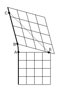
The grids we’ve been drawing are mere conventions, as elaborate and arbitrary as dress in the court of Louis XIV. They come from a surveying process, which may need to be planned in advance and whose results we might not be able to see until later. The dark line in figure \(\PageIndex{10}\) is the world-line of an observer \(O\), who moves inertially for a while, accelerates to the left, and then moves inertially again. On the right are pasted two coordinate grids adapted to the two inertial segments. At event \(E\), Bush steals the 2000 election, and this is depicted as being simultaneous with both event \(A\) and event \(B\). Does poor O see it happen twice? No, even if the bad news is transmitted by a signal moving at the speed of light (dashed line), \(O\) receives it only once, at event \(C\).

The only problem here is a poor choice of labels, which causes \(E\) to have more than one label. Something similar happens in a constant-acceleration frame, section 7.1,

Many mistakes by beginners at relativity revolve around a set of unexamined preconceptions about what it means to observe things. One imagines that effects such as length contraction and time dilation are what an observer actually sees, and perhaps that this process of seeing is instantaneous. Or one thinks of Minkowski coordinates as if they were the result of a simple and automatic process of perception by an observer. This is the kind of thinking that will lead one to believe that example \(\PageIndex{7}\) is crazy or paradoxical.

Figure \(\PageIndex{11}\): Minkowski coordinates are the result of a complicated process of surveying.

As another example, it should not be imagined that the length contraction of a stick by \(\frac{1}{\gamma}\) is what an observer actually sees when looking at the stick. Optical observations are influenced, for example, by the unequal times taken for light to propagate from the ends of the stick to the eye. A simulation of this type of effect is drawn in example 1.3.3.

Length contraction, time dilation, the observer-dependence of simultaneity, and Minkowski coordinates are all sophisticated results of a laborious process of collecting and analyzing data obtained by techniques such as Einstein synchronization, which require actions such as consulting atomic clocks or exchanging signals between different points at the speed of light. Figure \(\PageIndex{11}\) outlines such a process in a cartoonish way. A fleet of rocket ships, carrying surveyors, is sent out from Earth and dispersed throughout a vast region of space. Surveyors look through their theodolites at images, which are formed by light rays (dashed lines) that have arrived after traveling at the finite speed c. Such light rays carry old, stale information about various events. A nuclear war has broken out. Rock and roll music has arrived on Saturn. The resulting data are then transmitted by various means (passenger pigeon, Morse-coded radio, paper mail) and consolidated at the surveying office. At the office, workers at a long row of desks crunch the numbers and produce a chart of Minkowski coordinates with the events marked in.