2.5: Second Derivatives and Exact Differentials

If \(z = z(x , y)\), we can go through the motions of calculating \( \frac{\partial z}{\partial x}\) and \( \frac{\partial z}{\partial y}\), and we can then further calculate the second derivatives \( \frac{\partial ^2 z}{\partial x^2}\), \(\frac{\partial ^2 x}{\partial y^2}\), \( \frac{\partial ^2 z}{\partial y \partial x}\) and \(\frac{\partial ^2 z}{\partial y \partial x}\). It will usually be found that the last two, the mixed second derivatives, are equal; that is, it doesn’t matter in which order we perform the differentiations.

Example \(\PageIndex{1}\)

Let \(z = x \sin y\). Show that

\[ \dfrac{\partial ^2 z}{\partial x \partial y} = \dfrac{\partial ^2 z}{\partial y \partial x} = \cos y.\]

Solution

We examine in this section what conditions must be satisfied if the mixed derivatives are to be equal.

Figure II.1 depicts z as a “well-behaved” function of x and y. By “well-behaved” in this context I mean that z is everywhere single-valued (that is, given x and y there is just one value of z), finite and continuous, and that its derivatives are everywhere continuous (that is, no sudden discontinuities in either the function itself or its slope). “Good behaviour” in this sense is the sufficient condition that the mixed second derivatives are equal.

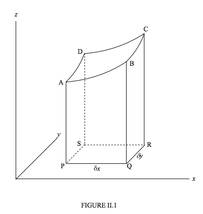
Let us calculate the difference δz in the heights of A and C. We can go from A to C via B or via D, and δz is route-independent. That is, to first order,

\[ \delta z = \left( \frac{\partial z}{\partial x} \right)_y^{ (A)} \delta x + \left( \frac{\partial z}{\partial y} \right)_x^{(B)} \delta y = \left( \frac{\partial z}{\partial y} \right)_x^{(A)} \delta y + \left( \frac{\partial z}{\partial x} \right)_y^{(D)} \delta x.\]

Here the superscript (A) means “evaluated at A”.

Divide both sides by δx δy:

\[ \frac{ \left( \frac{\partial z}{\partial y} \right)_x^{(B)} - \left( \frac{\partial z}{\partial y} \right)_x^{(A)}}{\partial x} = \frac{ \left( \frac{\partial z}{\partial x} \right)_y^{(D)} - \left( \frac{\partial z}{\partial x} \right)_y^{(A)}}{\partial y}.\]

If we now go to the limit as δx and δy approach zero (the equation now becomes exact rather than merely “to first order”), this becomes:

\[ \frac{\partial ^2 z}{\partial x \delta y} = \frac{\partial ^2 z}{\partial y \delta x}.\]

A further property of a function that is well-behaved in the sense described is that if the differential dz can be written in the form

\[ dz = A (x,~y) dx + B(x,~y) dy,\]

then Equation 2.5.3 implies that,

\[ \frac{\partial A}{\partial y} = \frac{\partial B}{\partial x}.\]

A differential dz is said to be exact if the following conditions are satisfied: The integral of dz between two points is route-independent, and the integral around a closed path (i.e. you end up where you started) is zero, and if equations 2.5.3 and 2.5.5 are satisfied.

If a differential such as Equation 2.5.4 is exact – i.e., if it is found to satisfy the conditions for exactness – then it should be possible to integrate it and determine z(x , y). Let us look at an example. Suppose that

\[ dz = (4x-3y-1)dx + (-3x+2y+4)dy.\]

It is readily seen that this is exact. The problem now, therefore, is to find z(x, y).

Let \( u = \int (4x - 3y - 1) dx\)

So that

\[ u = 2x^2 - 3yx - x + g(y).\]

Note that we are treating y as constant. The “constant” of integration depends on the value of y – i.e. it is an arbitrary function of y.

Of course u is not the same as z – unless we can find a particular function g(y) such that u indeed is the same as z.

Now \( du = \frac{\partial u}{\partial x} + \frac{\partial u}{\partial y} dy\); that is,

\[ du = (4x-3y-1)dx + \left( -3x + \frac{dg}{dy} \right) dy.\]

Then du = dz (and u = z plus an arbitrary constant) provided that \( \frac{dg}{dy} = 2y+4\). That is,

\[ g(y) = y^2 + 4y + \text{constant.}\]

Thus

\[ z = 2x^2 -3xy + y^2 -x + 4y + \text{constant}\]

The reader should verify that this satisfies equation 2.5.6. The reader should also try letting

\[ \nu = -3xy +y^2 + 4y + f(x)\]

(where did this come from?) and go through a similar argument to arrive again at equation 2.5.10.

Consider another example

Example \(\PageIndex{2}\)

\[ dz = 3 \ln y ~ dx + \frac{x}{y} dy.\]

You should immediately find that this differential is not exact, and, to emphasize that, I shall use the symbol đz, the special symbol đ indicating an inexact differential. However, given an inexact differential đz, it is very often possible to find a function H(x , y) such that the differential dw = H(x , y) đz is exact, and dw can then be integrated to find w as a function of x and y. The function H(x , y) is called an integrating factor. There may be more than one possible integrating factor; indeed it may be possible to find one simply of the form F(x) or maybe G(y). There are several ways for finding an integrating factor. We’ll do a simple and straightforward one. Let us try and find an integrating factor for the inexact differential đz above. Thus, let dw = F(x)dz, so that

\[ dw = 3F \ln y~ dx + \frac{xF}{y}dy.\]

For dw to be exact, we must have

\[ \frac{\partial }{\partial y} (3F \ln y) = \frac{\partial }{\partial x} \left( \frac{xF}{y} \right).\]

That is,

\[ \frac{3F}{y} = \frac{1}{y} \left( F + x \frac{dF}{dx} \right).\]

Upon integration and simplification we find that

\[ F = x^2,\]

or any multiple thereof, is an integrating factor, and therefore

\[ dw = 3x^2 \ln y~ dx + \frac{x^3}{y} dy\]

is an exact differential. The reader should confirm that this is an exact differential, and from there show that

\[ w = x^3 \ln y + \text{constant}\]

To anticipate – what has this to do with thermodynamics? To give an example, the state of many simple thermodynamical systems can be specified by giving the values of three intensive state variables, P, V and T, the pressure, molar volume and temperature. That is, the state of the system can be represented by a point in PVT space. Often, there will be a known relation (known as the equation of state) between the variables; for example, if the substance involved is an ideal gas, the variables will be related by PV = RT, which is the equation of state for an ideal gas; and the point representing the state of the system will then be represented by a point that is constrained to lie on the two-dimensional surface PV = RT in three-dimensional PVT space. In that case it will be necessary to specify only two of the three variables. On the other hand, if the equation of state of a particular substance is unknown, you will have to give the values of all three variables.

Now there are certain quantities that one meets in thermodynamics that are functions of state. Two that come to mind are entropy S and internal energy U. By function of state it is meant that S and U are uniquely determined by the state (i.e. by P, V and T). If you know P, V and T, you can calculate S and U or any other function of state. In that case, the differentials dS and dU are exact differentials.

The internal energy U of a system is defined in such a manner that when you add a quantity dQ of heat to a system and also do an amount of work dW on the system, the increase dU in the internal energy of the system is given by

\[dU = dQ + dW.\]

Here dU is an exact differential, but dQ and dW are clearly not. You can achieve the same increase in internal energy by any combination of heat and work, and the heat you add to the system and the work you do on it are clearly not functions of the state of the system.

Some authors like to use a special symbol, such as đ, to denote an inexact differential (but beware, I have seen this symbol used to denote an exact differential!). I shall not in general do this, because there are many contexts in which the distinction is not important, or, if it is, it is obvious from the context whether a given differential is exact or not. If, however, there is some context in which the distinction is important (and there are many) and in which it may not be obvious which is which, I may, with advance warning, use a special đ for an inexact differential, and indeed I have already done so earlier in this section.