Physics LibreTexts

4.4: The Heat Conduction Equation

  • Page ID
    7231
  • \( \newcommand{\vecs}[1]{\overset { \scriptstyle \rightharpoonup} {\mathbf{#1}} } \) \( \newcommand{\vecd}[1]{\overset{-\!-\!\rightharpoonup}{\vphantom{a}\smash {#1}}} \)\(\newcommand{\id}{\mathrm{id}}\) \( \newcommand{\Span}{\mathrm{span}}\) \( \newcommand{\kernel}{\mathrm{null}\,}\) \( \newcommand{\range}{\mathrm{range}\,}\) \( \newcommand{\RealPart}{\mathrm{Re}}\) \( \newcommand{\ImaginaryPart}{\mathrm{Im}}\) \( \newcommand{\Argument}{\mathrm{Arg}}\) \( \newcommand{\norm}[1]{\| #1 \|}\) \( \newcommand{\inner}[2]{\langle #1, #2 \rangle}\) \( \newcommand{\Span}{\mathrm{span}}\) \(\newcommand{\id}{\mathrm{id}}\) \( \newcommand{\Span}{\mathrm{span}}\) \( \newcommand{\kernel}{\mathrm{null}\,}\) \( \newcommand{\range}{\mathrm{range}\,}\) \( \newcommand{\RealPart}{\mathrm{Re}}\) \( \newcommand{\ImaginaryPart}{\mathrm{Im}}\) \( \newcommand{\Argument}{\mathrm{Arg}}\) \( \newcommand{\norm}[1]{\| #1 \|}\) \( \newcommand{\inner}[2]{\langle #1, #2 \rangle}\) \( \newcommand{\Span}{\mathrm{span}}\)\(\newcommand{\AA}{\unicode[.8,0]{x212B}}\)

    The situation described in Section 4.2 and in figure IV.1 was a steady-state situation, in which the temperature was a function of x but not of time. We are now going to consider a more general situation in which the temperature may vary in time as well as in space.

    Screen Shot 2019-06-28 at 5.13.45 PM.png

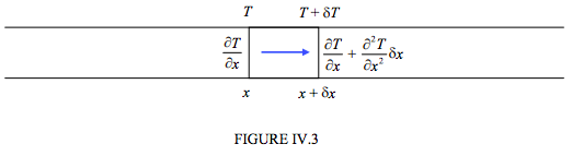
    In this case the temperature gradient is written as a partial derivative, \( \frac{\partial T}{\partial x} and is not uniform down the length of the rod. We'll suppose it is \frac{ \deta T}{\partial x} at x and \( \frac{\partial T}{\partial x} + \frac{\partial ^2 T}{\partial x^2} \delta x\) at x + δx.

    Consider the heat flow into and out of the portion between x and x + δx. The rate of flow into this portion at x is \( -KA \frac{\partial T}{\partial x}\), and the rate of flow out at x + δx is \( -KA \left( \frac{\partial T}{\partial x} + \frac{\partial ^2 T}{\partial x^2} \delta x \right)\), so that the net flow of heat into that portion is \( KA \frac{\partial ^2 T}{\partial x^2} \delta x\). This must be equal to \( C \rho A \delta x \frac{\partial T}{\partial t}\), where ρ is the density (and hence ρAδx is the mass of the portion), and C is the specific heat capacity.

    Therefore

    \[ C \rho \frac{\partial T}{\partial t} = K \frac{\partial ^2 T}{\partial x^2}.\]

    This can be written

    \[ \frac{\partial T}{\partial t} = D \frac{\partial ^2 T}{\partial x^2},\]

    where

    \[ D = \frac{K}{C \rho}\]

    is the thermal diffusivity (m2 s−1).

    Equation 4.3.2 is the heat conduction equation. In three dimensions it is easy to show that it becomes

    \[ T = D \nabla^2 T.\]


    This page titled 4.4: The Heat Conduction Equation is shared under a CC BY-NC license and was authored, remixed, and/or curated by Jeremy Tatum.

    • Was this article helpful?