4.5: A Solution of the Heat Conduction Equation

Methods of solving the heat conduction equation are commonly given in courses on partial differential equations. Here we shall look at a simple one-dimensional example.

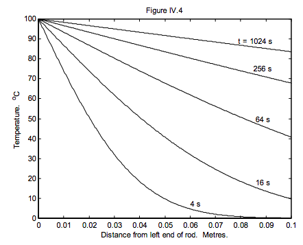
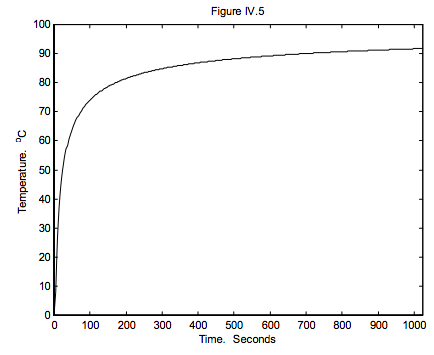
A long copper bar is initially at a uniform temperature of 0 ^oC. At time t = 0, the left hand end of it is heated to 100 ^oC. Draw graphs of temperature versus distance x from the hot end of the bar (up to x = 100 cm) at t = 4, 16, 64, 256 and 1024 seconds. Draw also a graph of temperature versus time at x = 5 cm, up to 1024 seconds. Assume no heat is lost from the sides of the bar.

Data for copper:

K = 400 W m⁻¹ K⁻¹

C = 395 J kg⁻¹ K⁻¹

ρ = 8900 kg m⁻³

whence

D = 1.137 × 10⁻⁴ m² s⁻¹

The equation to be solved is

$$D \frac{\partial ^2 T}{\partial x^2} = \frac{\partial T}{\partial t}$$

From the form of this equation, it is obvious (once it has been pointed out!) that a solution could be found in which T(x, t) is solely a function of x²/t, or, for that matter, x/t^1/2. Thus, let

$$u = x/t^{1/2},$$

and you will see that equation 4.4.1 reduces to the second order total differential equation

$$D \frac{d^2T}{du^2} = - \frac{u}{2} \frac{dT}{du}.$$

Let T' = dT/du, and it becomes even easier − a first order equation:

$$D \frac{dT'}{du} = - \frac{1}{2} uT'.$$

Upon integration, we obtain

$$\ln T' = - \frac{u^2}{4D} + \ln A,$$

where ln A is an integration constant, to be determined by the initial and boundary conditions. (What are the dimensions of A?)

That is,

$$T' = A \text{exp} \left[ -u^2 /(4D) \right].$$

We have to integrate again, with respect to u:

$$T = A \int \text{exp} \left[ - u^2/(4D) \right] du.$$

Now, T = 100 ^oC at x = 0 for any t > 0. That is, T = 100 for u = 0.

And T = 0 ^oC at t = 0 for any x > 0. That is, T = 0 for u = ∞.

Therefore

$$100 - 0 = A \int_{ \infty}^0 \text{exp} \left[ -u^2 /(4D) \right] du.$$

The integral is slightly difficult though well known. I'll just state the answer here; it is $- \sqrt{ \pi D}$. From this, we find that the integration constant is

$$A = -5284 \text{K m}^{-1} \text{s}^{1/2}.$$

We now have

$$100 - T (x,~t) = A \int_{xt^{-1/2}}^0 \text{exp} \left[ -u^2 /(4D) \right] du.$$

The error function erf(r) is defined by

$$\text{erf} (r) = \frac{2}{ \sqrt{ \pi}} \int_0^r \text{exp} (-s^2)ds,$$

so that equation 4.4.10 can be written

$$T (x,~t) = 100 + A \sqrt{ \pi D} \text{erf} \left( \frac{x}{ 2 \sqrt{Dt}} \right) = 100 \left[ 1 - \text{erf} \left( \frac{x}{2 \sqrt{Dt}} \right) \right].$$

This function is easy to plot provided that your computer will give you the erf function. The solutions are shown in figures IV.4 and 5.