2.7: Using Entropy to Find (Define) Temperature and Pressure

References: Schroeder sections 3.1, 3.4, and 3.5. Reif section 3.3. Kittel and Kroemer pages 30–41.

You will remember that one of the problems with our ensemble approach to statistical mechanics is that, while one readily sees how to calculate ensemble average values of microscopic (mechanical) quantities like the kinetic energy, the potential energy, or the mean particle height, it is hard to see how to calculate the sort of macroscopic (thermodynamic) quantity that we’re really more interested in anyway, such as the temperature or pressure. In fact, it is not even clear how we should define these important quantities. Our task in this lecture is to motivate such definitions. Because our arguments are motivations rather than deductions, they will be suggestive rather than definitive. The arguments can be made substantially more solid, but only at the cost of dramatic increase in mathematical complexity. (See David Ruelle’s Statistical Mechanics: Rigorous Results [Physics QC174.8.R84 1989].) At this stage in your education, you should just accept the arguments and the definitions, realizing that they are not definitive, and go on to learn how to use them. If you’re still worried about them a year from now, then that would be a good time to read the more complex arguments in Ruelle’s book.

An analogy will help explain the mathematical level of this lecture. Why is the period of the simple harmonic oscillator independent of amplitude? I can give two answers: 1) At larger amplitudes, the particle has more distance to move, but it also moves faster, and these two effects exactly cancel. 2) Solve the problem mathematically, and you’ll see that \(\omega = \sqrt{k/m}\) which is clearly unaffected by amplitude. The first answer gives more insight into what is going on physically, but it is not definitive. (It does not explain why the two effects cancel exactly rather that have one dominate the other, which is the case for non-parabolic oscillators.) The second argument is bulletproof, but it gives little insight. It is best to use both types of argument in tandem. Unfortunately, the bulletproof arguments for this section are really too elaborate and formal to present here. (In a few weeks I will give you a sample of a rigorous statistical mechanical argument: “The Grand Canonical Ensemble in the Thermodynamic Limit”, section 4.8. It is the easiest such argument that I know of, and you will see that it’s not very easy at all!)

Rapidly increasing character of the Ω(E) function

For a monatomic ideal gas (“in the thermodynamic limit”) the entropy is

\[S(E, V, N) \equiv k_{B} \ln \Omega(E, V, N)=k_{B} N\left[\frac{3}{2} \ln \left(\frac{4 \pi m E V^{2 / 3}}{3 h_{0}^{2} N^{5 / 3}}\right)+\frac{5}{2}\right].\]

Thus Ω(E, V, N), the number of microstates consistent with the macrostate (or thermodynamic state) specified by E, V, and N, is

\[\Omega(E, V, N)=e^{(5 / 2) N}\left(\frac{4 \pi m E V^{2 / 3}}{3 h_{0}^{2} N^{5 / 3}}\right)^{(3 / 2) N}.\]

In particular, as a function of energy,

\[\Omega(E)=(\text { constant }) E^{(3 / 2) N}.\]

This is a very rapidly increasing function of \(E\). (The function \(f(x) = x^2\) increases more rapidly than \(f(x) = x\). The function \(f(x) = x^3\) increases more rapidly than \(f(x) = x^2\). The function \(f(x) = x^{10^{23}}\) increases very rapidly indeed!) Although we have proven this result only for the ideal gas, it is plausible¹⁴ for interacting systems as well: If you throw more energy into a system, there are more ways for the energy to be arranged. (There is an argument to this effect in Reif’s section 2.5. The result is not, however, always true. . . check out the ideal paramagnet.)

As the particle number \(N\) grows larger and larger (approaching the “thermodynamic limit”) this increase of \(Ω\) with \(E\) becomes more and more rapid.

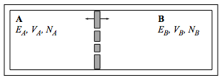
Two isolated systems

Consider two systems, \(A\) and \(B\), enclosed in our perfectly reflecting no-skid walls. System \(A\) has energy \(E_A\), volume \(V_A\), and particle number \(N_A\); similarly for system B.

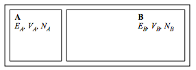
I have drawn the two systems adjacent, but they might as well be miles apart because they can’t affect each other through the no-skid walls. No energy can flow from one system to the other because no energy can move from the atoms in the system into the walls. The formal name for such walls is “insulating” or “adiabatic”. As we have discussed previously, such perfectly insulating walls do not exist in nature (if nothing else, system A affects system B through the gravitational interaction), but good experimental realizations exist and they are certainly handy conceptually.

The total system consisting of \(A\) plus \(B\) is characterized by the macroscopic quantities \(E_A\), \(E_B\), \(V_A\), \(V_B\), \(N_A\), and \(N_B\). The number of microstates corresponding to this macrostate is

\[Ω_T (E_A, E_B, V_A, V_B, N_A, N_B) = Ω_A(E_A, V_A, N_A)Ω_B(E_B, V_B, N_B).\]

Two systems in thermal contact

Consider the same two systems, \(A\) and \(B\), as before, but now allow the wall between them to be an ordinary, energy-permeable wall. Such a wall is called “diathermal”. (The walls between the systems and the outside world are still insulating.)

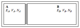
Now the mechanical parameters \(V_A, V_B, N_A\), and \(N_B\) still remain constant when the two systems are brought together, but the energies \(E_A\) and \(E_B\) change. (Of course the total energy \(E_T \equiv E_A + E_B\) remains constant as individual energies change.) Such contact between two systems, where energy can flow between the systems but where the mechanical parameters don’t change, is called “thermal contact”. Once they are in contact, I don’t know what the distribution of energy between \(A\) and \(B\) is: It could be that \(A\) is in its ground state and all the excess energy is in \(B\), or vice versa, and it could change rapidly from one such extreme to the other. But while I no longer have knowledge of the distribution, I do have an expectation. My expectation, drawn from daily experience, is that energy will flow from one system to another until \(E_A\) and \(E_B\) take on some pretty well-defined final equilibrium values. The exact energies will then fluctuate about those equilibrium values, but those fluctuations will be small. And what characterizes this final equilibrium situation? Your first guess might be that the energy on each side should be equal. But no, if a big system were in contact with a small system, then you’d expect more energy to end up in the big system. Then you might think that the energy per particle on each side should be equal, but that’s not right either. (Ice and liquid water are in equilibrium at the freezing point, despite the fact that the energy per particle of liquid water is much greater than than of ice.) The correct expectation (known to any cook) is that:

When two systems \(A\) and \(B\) are brought into thermal contact, \(E_A\) and \(E_B\) will change until they reach equilibrium values \(E^{(e)}_A\) and \(E^{(e)}_B\), with negligible fluctuations, and at equilibrium both systems \(A\) and \(B\) will have the same “temperature”.

This is the qualitative property of temperature that will allow us, in a few moments, to produce a rigorous, quantitative definition. To do so we now look at the process microscopically instead of through our macroscopic expectations.

Once the two systems are in thermal contact the energy of system A could be anything from 0 to the total energy \(E_T\)¹⁵ For any given \(E_A\), the number of accessible microstates of the combined system, \(A\) plus \(B\), is \(Ω_A(E_A)Ω_B(E_T − E_A)\). Thus the total number of microstates of the combined system is

\[\Omega_{T}\left(E_{T}\right)=\sum_{E_{A}=0}^{E_{T}} \Omega_{A}\left(E_{A}\right) \Omega_{B}\left(E_{T}-E_{A}\right).\]

(Please don’t tell me the obvious. . . that \(E_A\) is a continuous quantity so you have to integrate rather than sum. This is a seat-of-the-pants argument. If you want attention to fine points, look them up in Ruelle’s book.) Let us examine the character of the summand, \(Ω_A(E_A)Ω_B(E_T −E_A)\), as a function of \(E_A\). The functions \(Ω_A(E_A)\) and \(Ω_B(E_B)\) are both rapidly increasing functions of their arguments, so \(Ω_B(E_T − E_A)\) is a rapidly decreasing function of \(E_A\). Thus the product \(Ω_A(E_A)Ω_B(E_T − E_A)\) will start out near zero, then jump up for a narrow range of EA values and then fall quickly to near zero again.

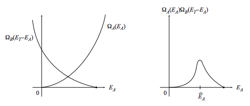
In conclusion, for most values of \(E_A\) the summand nearly vanishes, so most of the contribution to the sum comes from its largest term, which is located at an energy we will call \( \hat{E}_A\):

\[\Omega_{T}\left(E_{T}\right)=\Omega_{A}\left(\hat{E}_{A}\right) \Omega_{B}\left(E_{T}-\hat{E}_{A}\right)+\text { small change. }\]

The sharply peaked character of the product \(Ω_A(E_A)Ω_B(E_T − E_A)\) becomes more and more pronounced as the thermodynamic limit is approached, so in this limit the “small change” can be ignored. You can see that for macroscopic systems the “microscopically most probable value” \( \hat{E}_A\) should be interpreted as the thermodynamic equilibrium value \(E^{(e)}_A\).

We locate this value by maximizing

\[\Omega_{A}\left(E_{A}\right) \Omega_{B}\left(E_{T}-E_{A}\right).\]

To make life somewhat easier, we will not maximize this function directly but, what is the same thing, maximize its logarithm

\[f\left(E_{A}\right) \equiv \ln \left[\Omega_{A}\left(E_{A}\right) \Omega_{B}\left(E_{T}-E_{A}\right)\right]\]

\[=\ln \Omega_{A}\left(E_{A}\right)+\ln \Omega_{B}\left(E_{T}-E_{A}\right).\]

Recognizing the entropy terms we have

\[ k_{B} f\left(E_{A}\right)=S_{A}\left(E_{A}\right)+S_{B}\left(E_{T}-E_{A}\right),\]

and differentiation produces

\[\frac{\partial\left(k_{B} f\left(E_{A}\right)\right)}{\partial E_{A}}=\frac{\partial S_{A}}{\partial E_{A}}+\frac{\partial S_{B}}{\partial E_{B}} \frac{\frac{\partial E_{B}}{\partial E_{A}}}{\underbrace{\partial E_{A}}_{-1}}.\]

We locate the maximum by setting the above derivative to zero, which tells us that at equilibrium

\[ \frac{\partial S_{A}}{\partial E_{A}}=\frac{\partial S_{B}}{\partial E_{B}}.\]

Our expectation is that the temperature will be the same for system \(A\) and system \(B\) at equilibrium, while our microscopic argument shows that \(∂S/∂E\) will be the same for system \(A\) and system \(B\) at equilibrium. May we conclude from this that

\[ \frac{\partial S}{\partial E}=\text { Temperature ? }\]

No we cannot! All we can conclude is that

\[ \frac{\partial S}{\partial E}=\text { invertible function (Temperature) }.\]

To find out which invertible function to choose, let us test these ideas for the ideal gas. Using

\[S(E)=k_{B} \ln C+\frac{3}{2} k_{B} N \ln E+\frac{5}{2} k_{B} N\]

we find

\[\frac{\partial S}{\partial E}=\frac{3}{2} k_{B} \frac{N}{E},\]

so a large value of \(E\) results in a small value of \(∂S/∂E\). Because we are used to thinking of high temperature as related to high energy, it makes sense to define (absolute) temperature through

\[ \frac{1}{T(E, V, N)} \equiv \frac{\partial S(E, V, N)}{\partial E}.\label{2.56}\]

Note

Applying this definition to the ideal gas gives the famous result

\[ \frac{E}{N}=\frac{3}{2} k_{B} T.\label{2.57}\]

In fact, this result is too famous, because people often forget that it applies only to a classical monatomic ideal gas. It is a common misconception that temperature is defined through Equation \ref{2.57} rather than through Equation \ref{2.56}, so that temperature is always proportional to the average energy per particle or to the average kinetic energy per particle. If this misconception were correct, then when ice and water were in equilibrium, the molecules in the ice and the molecules in the water would have the same average energy per particle! In truth, these proportionalities hold exactly only for noninteracting classical point particles.

Two systems in thermal and mechanical contact

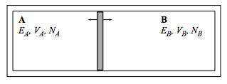
Consider the same two systems, \(A\) and \(B\), as before, but now allow them to exchange both energy and volume. (The wall between \(A\) and \(B\) is a sliding, diathermal wall. The walls between the systems and the outside world remains insulating and rigid.)

The dimensions of \(∂S/∂V\) are

\[ \left[\frac{\partial S}{\partial V}\right]=\frac{\mathrm{J} / \mathrm{K}}{\mathrm{m}^{3}}\]

while those for pressure are

\[[p]=\frac{\mathrm{J}}{\mathrm{m}^{3}}.\]

This motivates us to define pressure through

\[\frac{p(E, V, N)}{T(E, V, N)} \equiv \frac{\partial S(E, V, N)}{\partial V}.\]

Note

For an ideal gas,

\[ S(V)=k_{B} N[C+\ln V].\]

so

\[ \frac{\partial S}{\partial V}=\frac{k_{B} N}{V}=\frac{p}{T},\]

leading to

\[ p V=N k_B T,\]

the ideal gas equation of state! (Which is again too famous for its own good. Too many statistical mechanics courses degenerate into “an intensive study of the ideal gas”, and it is a shame to waste such a beautiful, powerful, and diverse subject on the study of only one substance, especially since that substance doesn’t even exist in nature!)

Two systems that can exchange energy, volume, and particles

We return to the same situation as before, but now the wall between \(A\) and \(B\) is not only diathermal and sliding, but also allows particles to flow. (Imagine piercing a few tiny holes in the wall.)

The reasoning in this case exactly parallels the reasoning already given two above, so I will not belabor it. I will merely point out that we can now define a new quantity, the chemical potential \(\mu\), which governs the flow of particles just as temperature governs the flow of energy or pressure governs the flow of volume. It is

\[-\frac{\mu(E, V, N)}{T(E, V, N)} \equiv \frac{\partial S(E, V, N)}{\partial N}.\]

The meaning of chemical potential

The upshot of all our definitions is that

\[d S=\frac{1}{T} d E+\frac{p}{T} d V-\frac{\mu}{T} d N.\]

What do these definitions mean physically? The first term says that if two systems are brought together so that they can exchange energy but not volume or particle number, then in the system with high temperature the energy will decrease while in the system with low temperature the energy will increase. The second term says that if two systems with the same temperature are brought together so that they can exchange volume but not particle number, then in the system with high pressure the volume will increase while in the system with low pressure the volume will decrease. The third term says that if two systems with the same temperature and pressure are brought together so that they can exchange particles, then in the system with high chemical potential the number will decrease while in the system with low chemical potential the number will increase. In summary:

Exchange of energy?	Exchange of volume?	Exchange of particles?	Result:
Yes Permitted, but \(∆T = 0\). Permitted, but \(∆T = 0\).	Prohibited. Yes. Permitted, but \(∆p = 0\).	Prohibited. Prohibited. Yes.	System with high \(T\) decreases in \(E\). System with high \(p\) increases in \(V\). System with high \(\mu\) decreases in \(N\).

Chemists have a great name for chemical potential. . . they call it “escaping tendency”, because particles tend to move from a region of high \(\mu\) to a region of low \(\mu\) just as energy tend to move from a region of high \(T\) to a region of low \(T\). (G.W. Castellan, Physical Chemistry, 2nd edition, Addison-Wesley, Reading, Mass., 1971, section 11–2.) You can see that chemical potential is closely related to density, and indeed for an ideal gas

\[ \mu=k_{B} T \ln \left(\lambda^{3}(T) \rho\right),\]

where \(ρ = N/V\) is the number density and \(\lambda(T)\) is a certain length, dependent upon the temperature, that we will see again (in equation (5.4)).

Note

Once again, remember that this relation holds only for the ideal gas. At the freezing point of water, when ice and liquid water are in equilibrium, the chemical potential is the same for both the solid and the liquid, but the densities clearly are not!

Problems

2.21 (Q) The location of \(E_A^{(e)}\)

In the figure on page 41, does the equilibrium value \(E_A^{(e)}\) fall where the two curves \(Ω_A(E_A)\) and \(Ω_B(E_T − E_A)\) cross? If not, is there a geometrical interpretation, in terms of that figure, that does characterize the crossing?

2.22 (Q) Meaning of temperature and chemical potential

The energy of a microscopic system can be dissected into its components: the energy due to motion, the energy due to gravitational interaction, the energy due to electromagnetic interaction. Can the temperature be dissected into components in this way? The chemical potential? (Clue: Because the temperature and chemical potential are derivatives of the entropy, ask yourself first whether the entropy can be dissected into components.)

2.23 (E) Chemical potential of an ideal gas

a. Show that the chemical potential of a pure classical monatomic ideal gas is

\[\mu=-\frac{3}{2} k_{B} T \ln \left(\frac{4 \pi m E V^{2 / 3}}{3 h_{0}^{2} N^{5 / 3}}\right)\]

\[ =-k_{B} T \ln \left[\left(\frac{2 \pi m k_{B} T}{h_{0}^{2}}\right)^{3 / 2} \frac{V}{N}\right].\]

b. Show that when the temperature is sufficiently high and the density sufficiently low (and these are, after all, the conditions under which the ideal gas approximation is valid) the chemical potential is negative.

c. Show that

\[\frac{\partial \mu(T, V, N)}{\partial T}=\frac{\mu(T, V, N)}{T}-\frac{3}{2} k_{B}.\]

At a fixed, low density, does \(\mu\) increase or decrease with temperature?

2.24 Ideal paramagnet, take three

Find the chemical potential \(\mu(E, H, N)\) of the ideal paramagnet. (Your answer must not be a function of \(T\).) (To work this problem you must have already worked problems 2.9 and 2.12.)

Resources

Percival as CM for chaos and SM. Hilborn on chaos.

PAS chaos programs, public domain stadium and wedge. CUPS stadium.

Tolman, Ruelle.

¹⁴Through the booty argument of page 27.

¹⁵Here and in the rest of this section, we assume that the ground state energy of both system \(A\) and system \(B\) has been set by convention to zero.