
8.4: Applications of the Bose-Einstein Distribution


- Last updated
- Mar 28, 2021
- Save as PDF

( \newcommand{\kernel}{\mathrm{null}\,}\)
We shall now consider some simple applications of quantum statistics, focusing in this section on the Bose-Einstein distribution.
8.3.1: The Planck Distribution for Black Body Radiation
Any material body at a finite nonzero temperature emits electromagnetic radiation, or photons in the language of the quantum theory. The detailed features of this radiation will depend on the nature of the source, its atomic composition, emissivity, etc. However, if the source has a sufficiently complex structure, the spectrum of radiation is essentially universal. We want to derive this universal distribution, which is also known as the Planck distribution.
Since a black body absorbs all radiation falling on it, treating all wavelengths the same, a black body may be taken as a perfect absorber. (Black bodies in reality do this only for a small part of the spectrum, but here we are considering the idealized case.) By the same token, black bodies are also perfect emitters and hence the formula for the universal thermal radiation is called the black body radiation formula.
The black body radiation formula was obtained by Max Planck by fitting to the observed spectrum. He also spelled out some of the theoretical assumptions needed to derive such a result and this was, as is well known, the beginning of the quantum theory. Planck’s derivation of this formula is fairly simple once certain assumptions, radical for his time, are made; from the modern point of view it is even simpler. Photons are particles of zero rest mass, the energy and momentum of a photon are given as
ϵ=ħω,→p=ħ→k
where the frequency of the radiation ω and the wave number →k are related to each other in the usual way, ω=c|→k|. Further photons are spin-1 particles, so we know that they are bosons. Because they are massless, they have only two polarization states, even though they have spin equal to 1. (For a massive particle we should expect (2s+1)=3 polarization states for a spin-1 particle.) We can apply the Bose-Einstein distribution Equation 8.1.10 directly, with one caveat. The number of photons is not a well-defined concept. Since long-wavelength photons carry very little energy, the number of photons for a state of given energy could have an ambiguity of a large number of soft or long-wavelength photons. This is also seen more theoretically; there is no conservation law in electromagnetic theory beyond the usual ones of energy and momentum. This means that we should not have a chemical potential which is used to fix the number of photons. Thus the Bose-Einstein distribution simplifies to
n=1eβϵ−1
We now consider a box of volume V in which we have photons in thermal equilibrium with material particles such as atoms and molecules. The distribution of the internal energy as a function of momentum is given by
dU=2d3xd3p(2πħ)3ϵeβϵ−1
where the factor of 2 is from the two polarization states. Using Equation ???, for the energy density, we find
du=2d3k(2π)3ħωeħωkT−1
This is Planck’s radiation formula. If we use ω=c|→k| and carry out the integration over angular directions of →k, it reduces to
du=ħπ2c3dωω3eħωkT−1
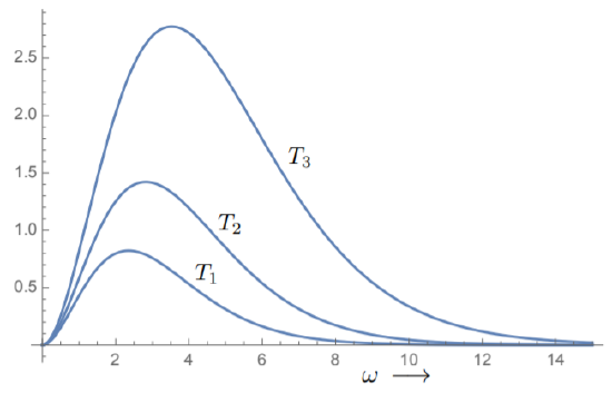
This distribution function vanishes at ω=0 and as ω→∞. It peaks at a certain value which is a function of the temperature. In Fig. 8.3.1, we show the distribution for some sample values of temperature. Note that the value of ω at the maximum increases with temperature; in addition, the total amount of radiation (corresponding to the area under the curve) also increases with temperature.
If we integrate ??? over all frequencies, the total energy density comes out to be
u=π215(ħc)3(kT)4
where we have used the result
∫∞0dxx3ex−1=3!ζ(4)=π415
Rate of Radiation from a Black Body
We can convert the formula for the energy density to the intensity of the radiation by considering the conservation of energy in electrodynamics. The energy density of the electromagnetic field is given by
u=12(E2+B2)
Using the Maxwell equations in free space, we find
∂u∂t=Ei˙Ei+Bi˙Bi=c[Ei(∇×B)i−Bi(∇×E)i]=−c∇⋅(→E×→B)=−∇⋅→P→P=c(→E×→B)
Integrating over a volume V, we find
∂∂t=∫d3xu=∮∂V→P⋅d→S
Thus the energy flux per unit area or the intensity is given by the Poynting vector →P=c(→E×→B). For electromagnetic waves, |E|=|B|, →E and →B are orthogonal to each other and both are orthogonal to →k, the wave vector which gives the direction of propagation, i.e., the direction of propagation of the photon. In this case we find
u=E2,→P=cuˆk
Using the Planck formula ???, the magnitude of the intensity of blackbody radiation is given by
dI=2cd3k(2π)3ħωeħωkT−1
We have considered radiation in a box of volume V in equilibrium. To get the rate of radiation per unit area of a blackbody, note that, because of equilibrium, the radiation rate from the body must equal the energy flux falling on area under consideration (which is all taken to be absorbed since it is a blackbody); thus emission rate equals absorption rate as expected for equilibrium. The flux is given by
→P⋅d→S=→P⋅ˆndS=cuˆk⋅ˆndS=cucosθdS
where ˆn is the normal to the surface and θ is the angle between ˆk and ˆn. Further, in the equilibrium situation, there are photons going to and away from the surface under consideration, so we must only consider positive values of ˆk⋅ˆn=cosθ, or 0≤θ≤π2. Thus the radiation rate over all wavelengths per unit area of the emitter is given by
R=2c∫d3k(2π)3ħωcosθeħωkT−1=2c∫dkk24π2ħωeħωkT−1∫π20dθsinθcosθ=ħ4π2c2∫∞0dωω3eħωkT−1=σT4σ=π2k460ħ3c2
This result is known as the Stefan-Boltzmann law.
Radiation Pressure
Another interesting result concerning thermal radiation is the pressure of radiation. For this, it is convenient to use one of the relations in Equation 6.2.21, namely,
(∂U∂V)T=T(∂p∂T)V−p
From Equation ???, we have
U=Vπ215(ħc)3k4T4
Equations ??? and ??? immediately lead to
p=π245(ħc)3k4T4=13u
Radiation pressure is significant and important in astrophysics. Stars can be viewed as a gas or fluid held together by gravity. The gas has pressure and the pressure gradient between the interior of the star and the exterior region tends to create a radial outflow of the material. This is counteracted by gravity which tends to contract or collapse the material. The hydrostatic balance in the star is thus between gravity and pressure gradients. The normal fluid pressure is not adequate to prevent collapse. The radiation produced by nuclear fusion in the interior creates an outward pressure and this is a significant component in the hydrostatic equilibrium of the star. Without this pressure a normal star would rapidly collapse.
Maximum of Planck Distribution
We have seen that the Planck distribution has a maximum at a certain value of ω. It is interesting to consider the wavelength λ∗ at which the distribution has a maximum. This can be done in terms of frequency or wavelength, but we will use the wavelength here as this is more appropriate for the application we consider later. (The peak for frequency and wavelength occur at different places since these variables are not linearly related, but rather are reciprocally related.) Using dω=−(2πc)dλλ2, we can write down the Planck distribution (Equation ???) in terms of the wavelength λ as
dI=2(2πħ)c21λ5(eħωkT−1)dλdΩ
(The minus sign in dω only serves to show that when the intensity increases with frequency, it should decrease with λ and vice versa. So we have dropped the minus sign. Ω is the solid angle for the angular directions.) Extremization with respect to λ gives the condition
(x-5)e^x + 5 = 0
where x = βħω. The solution of this transcendental equation is
λ_∗ \approx \frac{(2 \pi ħ)c}{k} \frac{1}{4.96511} \frac{1}{T} \label{8.3.20}
This relation is extremely useful in determining the temperature of the outer layer of stars, called the photosphere, from which we receive radiation. By spectroscopically resolving the radiation and working out the distribution as a function of wavelength, we can see where the maximum is, and this gives, via Equation \ref{8.3.20}, the temperature of the photosphere. Notice that higher temperatures correspond to smaller wavelengths; thus blue stars are hotter than red stars. For the Sun, the temperature of the photosphere is about 5777 K, corresponding to a wavelength λ_∗ ≈ 502 nm. Thus the maximum for radiation from the Sun is in the visible region, around the color green.
Another case of the importance in which the radiation pressure and the λ_∗ we calculated are important is in the early history of the universe. Shortly after the Big Bang, the universe was in a very hot phase with all particles having an average energy so high that their masses could be neglected. The radiation pressure from all these particles, including the photon, is an important ingredient in solving the Einstein equations for gravity to work out how the universe was expanding. As the universe cooled by expansion, the unstable massive particles decayed away, since there was not enough average energy in collisions to sustain the reverse process. Photons continued to dominate the evolution of the universe. This phase of the universe is referred to as the radiation-dominated era.
Later, the universe cooled enough for electrons and nuclei to combine to form neutral atoms, a phase known as the recombination era. Once this happened, since neutral particles couple only weakly (through dipole and higher multipole moments) to radiation, the existing radiation decoupled and continued to cool down independently of matter. This is the matter dominated era in which we now live. The radiation obeyed the Planck spectrum at the time of recombination, and apart from cooling would continue to do so in the expanding universe. Thus the existence of this background relic radiation is evidence for the Big Bang theory. This cosmic microwave background radiation was predicted to be a consequence of the Big Bang theory, by Gamow, Dicke and others in the 1940s. The temperature was estimated in calculations by Alpher and Herman and by Gamow in the 1940s and 1950s. The radiation was observed by Penzias and Wilson in 1964. The temperature of this background can be measured in the same way as for stars, by comparing the maximum of the distribution with the formula \ref{8.3.20}. It is found to be approximately 2.7 K. (Actually this has been measured with great accuracy by now, the latest value being 2.72548 ± 0.00057 K). The corresponding λ_∗ is in the microwave region, which is why this is called the cosmic microwave background.
8.3.2: Bose-Einstein Condensation
We will now work out some features of an ideal gas of bosons with a conserved particle number; in this case, we do have a chemical potential. There are many atoms which are bosons and, if we can neglect the interatomic forces as a first approximation, this discussion can apply to gases made of such atoms. The partition function Z for gas of bosons was given in Equation 8.1.15. Since log Z is related to pressure as in Equation 7.4.19, this gives immediately
\begin{equation} \begin{split} \frac{pV}{kT} & = \log Z = - \int \frac{d^3x d^3p}{(2 \pi ħ)^3 \log \left( 1-e^{-\beta (\epsilon - \mu)} \right)} \\[0.125in] & = V \left( \frac{mkT}{2 \pi ħ^2} \right)^{\frac{3}{2}} \left[ z+ \frac{z^2}{2^\frac{5}{2}} + \frac{z^3}{3^\frac{5}{2}} + · · · \right] \\[0.125in] & = V \left( \frac{mkT}{2 \pi ħ^2} \right)^{\frac{3}{2}} \text{Li}_\frac{5}{2} (z) \\[0.125in] \end{split} \end{equation} \label{8.3.21}
where z = e βµ is the fugacity and \text{Li}_s(z) denotes the polylogarithm defined by
\text{Li}_s(z) = \sum_{n=1}^{\infty} \frac{z^n}{n^s}
The total number of particles N is given by the normalization condition (Equation 8.1.12) and works out to
\begin{equation} \begin{split} \frac{N}{V} & = \left( \frac{mkT}{2 \pi ħ^2} \right)^{\frac{3}{2}} \left[ z+ \frac{z^2}{2^\frac{3}{2}} + \frac{z^3}{3^\frac{3}{2}} + · · · \right] \\[0.125in] & = \left( \frac{mkT}{2 \pi ħ^2} \right)^{\frac{3}{2}} \text{Li}_\frac{3}{2} (z) = \frac{1}{λ^3} \text{Li}_{\frac{3}{2} (z)} \end{split} \end{equation} \label{8.3.23}
We have defined the thermal wavelength λ by
λ = \sqrt{\frac{2 \pi ħ^2}{mkT}}
Apart from some numerical factors of order 1, this is the de Broglie wavelength for a particle of energy kT.
If we eliminate z in favor of \frac{N}{V} from this equation and use it in Equation \ref{8.3.21}, we get the equation of state for the ideal gas of bosons. For high temperatures, this can be done by keeping the terms up to order z^2 in the polylogarithms. This gives
p = \frac{N}{V}kT \left[ 1- \frac{N}{V} \frac{λ^3}{2^{\frac{5}{2}}} + · · · \right]
This equation shows that even the perfect gas of bosons does not follow the classical ideal gas law. In fact, we may read off the second virial coefficient as
B_2 = - \frac{λ^3}{2^{\frac{5}{2}}} \label{8.3.26}
The thermal wavelength is small for large T, so this correction is small at high temperatures, which is why the ideal gas was a good approximation for many of the early experiments in thermal physics. If we compare this with the second virial coefficient of a classical gas with interatomic potential V (x) as given in Equation 7.5.11, namely,
B_2 = \frac{1}{2} \int d^3x \left( 1- e^{- \beta V(x)} \right)
we see that we can mimic Equation ref{8.3.26} by an attractive (V (x) < 0) interatomic potential. Thus bosons exhibit a tendency to cluster together.
We can now consider what happens when we lower the temperature. It is useful to calculate a typical value of λ. Putting in the constants,
λ = \sqrt{\left( \frac{300}{T} \right) \left( \frac{m_p}{m} \right) } \times 6.3 \times 10^{-10} \text{ meters} \label{8.3.28}
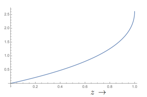
(m_p is the mass of the proton ≈ the mass of the hydrogen atom.) Thus for hydrogen at room temperature, λ is of atomic size. Since \frac{V}{N} is approximately the free volume available to a molecule, we find from Equation \ref{8.3.23} that z must be very small under normal conditions. The function Li_{\frac{3}{2}} (z) starts from zero at z = 0 and rises to about 2.61238 at z = 1, see Fig. 8.3.2. Beyond that, even though the function can be defined by analytic continuation, it is imaginary. In fact, there is a branch cut from z = 1 to ∞. Thus for z < 1, we can solve Equation \ref{8.3.23} for zin terms of \frac{N}{V}. As the temperature is lowered, λ decreases and eventually we get to the point where z = 1. This happens at a temperature
T_c = \frac{1}{k} \left( \frac{N}{V\;2.61238} \right)^{\frac{2}{3}} \left( \frac{2 \pi ħ^2}{m} \right) \label{8.3.29}
If we lower the temperature further, it becomes impossible to satisfy Equation \ref{8.3.23}. We can see the problem at z = 1 more clearly by considering the partition function, where we separate the contribution due to the zero energy state,
Z = \frac{1}{1-z} \prod_{p \neq 0} \frac{1}{1-ze^{-\beta \epsilon_p}}
We see that the partition function has a singularity at z = 1. This is indicative of a phase transition. The system avoids the singularity by having a large number of particles making a transition to the state of zero energy and momentum. Recall that the factor \frac{1}{(1 − z}) may be viewed as \sum_n z^n, as a sum over different possible occupation numbers for the ground state. The idea here is that, instead of various possible occupation numbers for the ground state, what happens below T_c is that there is a certain occupation number for the ground state, say, N_0, so that the partition function should read
Z = z^{N_0} \prod_{p \neq 0} \frac{1}{1-ze^{-\beta \epsilon_p}}
Thus, rather than having different probabilities for the occupation numbers for the ground state, with correspondingly different probabilities as given by the Boltzmann factor, we have a single multiparticle quantum state, with occupation number N_0, for the ground state. The normalization condition Equation \ref{8.3.23} is then changed to
\frac{N}{V} = \frac{N_0}{V} + \frac{1}{λ^3} \text{Li}_{\frac{3}{2}} (z) \label{8.3.32}
Below T_c, this equation is satisfied, with z = 1, and with N_0 compensating for the second term on the right hand side as λ increases. This means that a macroscopically large number of particles have to be in the ground state. This is known as Bose-Einstein condensation. In terms of T_c, we can rewrite Equation \ref{8.3.32} as
\frac{N_0}{V} = \frac{N}{V} + \left[1 - \left( \frac{T}{T_C} \right)^{\frac{3}{2}} \right] \label{8.3.33}
which gives the fraction of particles which are in the ground state.
Since z = 1 for temperatures below T_c, we have µ = 0. This is then reminiscent of the case of photons where we do not have a conserved particle number. The proper treatment of this condensation effect requires quantum field theory, using the concept of spontaneous symmetry breaking. In such a description, it will be seen that the particle number is still a conserved operator but that the condensed state cannot be an eigenstate of the particle number.
There are many other properties of the condensation phenomenon we can calculate. Here we will focus on just the specific heat. The internal energy for the gas is given by
\begin{equation} \begin{split} U & = \int \frac{d^3x d^3p}{(2 \pi ħ)^3} \frac{\epsilon}{e^{\beta (\epsilon - \mu)} - 1} \\[0.125in] & = V \frac{3}{2}kT \frac{1}{λ^3} \text{Li}_{\frac{5}{2}} (z) \end{split} \end{equation}
At high temperatures, z is small and \text{Li}_{\frac{5}{2}} (z) ≈ z and Equation \ref{8.3.23} gives \frac{z}{λ^3} = \frac{N}{V}. Thus U = \frac{3}{2}N kT in agreement with the classical ideal gas. This gives C_v = \left( \frac{3}{2} \right) N k.
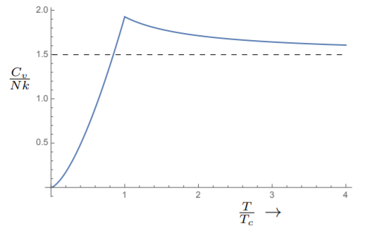
For low temperatures below T_c, z = 1 and we can set \text{Li}_{\frac{5}{2}} (z) = \text{Li}_{\frac{5}{2}} (1) ≈ 1.3415. The specific heat becomes
C_v = V\;k \frac{15}{4} \frac{ \text{Li}_{\frac{5}{2}} (1) }{λ^3} = N\;k \frac{15}{4} \frac{ \text{Li}_{\frac{5}{2}} (1) }{\text{Li}_{\frac{5}{2}} (1)} \left( \frac{T}{T_c} \right)^{\frac{3}{2}} ≈ 1.926\;N\;k\; \left( \frac{T}{T_c} \right)^{\frac{3}{2}}
We see that the specific heat goes to zero at absolute zero, in agreement with the third law of thermodynamics. It rises to a value which is somewhat above \frac{3}{2} at T = T_c. Above T_c, we must solve for z in terms of N and substitute back into the formula for U. But qualitatively, we can see that the specific heat has to decrease for T > T_c reaching the ideal gas value of \frac{3}{2} at very high temperatures. A plot of the specific heat is shown in Fig. 8.3.3.
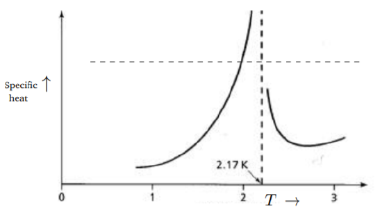
There are many examples of Bose-Einstein condensation by now. The formula for the thermal wavelength in Equation \ref{8.3.28} shows that smaller atomic masses will have larger λ and one may expect them to undergo condensation at higher temperatures. While molecular hydrogen (which is a boson) may seem to be the best candidate, it turns to a solid at around 14 \;K. The best candidate is thus liquid Helium. The atoms of the isotope \text{He}^4 are bosons. Helium becomes a liquid below 4.2 K and it has a density of about 125 \frac{kg}{m^3} (under normal atmospheric pressure) and if this value is used in the formula \ref{8.3.29}, we find T_c to be about 3\; K. What is remarkable is that liquid Helium undergoes a phase change at 2.17\; K. Below this temperature, it becomes a superfluid, exhibiting essentially zero viscosity. (He3 atoms are fermions, there is superfluidity here too, at a much lower temperature, and the mechanism is very different.) This transition can be considered as an example of Bose-Einstein condensation. Helium is not an ideal gas of bosons, interatomic forces (particularly a short-range repulsion) are important and this may explain the discrepancy in the value of T_c. The specific heat of liquid \text{He}_4 is shown in Fig. 8.3.4. There is a clear transition point, with the specific heat showing a discontinuity in addition to the peaking at this point. Because of the similarity of the graph to the Greek letter λ, this is often referred to as the λ-transition. The graph is very similar, in a broad qualitative sense, to the behavior we found for Bose-Einstein condensation in Fig. 8.3.3; however, the Bose-Einstein condensation in the noninteracting gas is a first-order transition, while the λ-transition is a second-order transition, so there are differences with the Bose-Einstein condensation of perfect gas of bosons.
The treatment of superfluid Helium along the lines we have used for a perfect gas is very inadequate. A more sophisticated treatment has to take account of interatomic forces and incorporate the idea of spontaneous symmetry breaking. By now, there is a fairly comprehensive theory of liquid Helium.
Recently, Bose-Einstein condensation has been achieved in many other atomic systems such as a gas of \text{Rb}^87 atoms, \text{Na}^23 atoms, and a number of others, mostly alkaline and alkaline earth elements.
8.3.3: Specific Heats of Solids
We now turn to the specific heats of solids, along the lines of work done by Einstein and Debye. In a solid, atoms are not free to move around and hence we do not have the usual translational degrees of freedom. Hence the natural question which arises is: When a solid is heated, what are the degrees of freedom in which the energy which is supplied can be stored? As a first approximation, atoms in a solid may be taken to be at the sites of a regular lattice. Interatomic forces keep each atom at its site, but some oscillation around the lattice site is possible. This is the dynamics behind the elasticity of the material. These oscillations, called lattice vibrations, constitute the degrees of freedom which can be excited by the supplied energy and are thus the primary agents for the specific heat capacity of solids. In a conductor, translational motion of electrons is also possible. There is thus an electronic contribution to the specific heat as well. This will be taken up later; here we concentrate on the contribution from the lattice vibrations. In an amorphous solid, a regular lattice structure is not obtained throughout the solid, but domains with regular structure exist, and so, the elastic modes of interest are still present.

Turning to the details of the lattice vibrations, for N atoms on a lattice, we expect 3N modes, since each atom can oscillate along any of the three dimensions. Since the atoms are like beads on an elastic string, the oscillations can be transferred from one atom to the next and so we get traveling waves. We may characterize these by a frequency ω and a wave number \vec{k}. The dispersion relation between ω and \vec{k} can be obtained by solving the equations of motion for N coupled particles. There are distinct modes corresponding to different ω-k relations; the typical qualitative behavior is shown in Fig. 8.3.5. There are three acoustic modes for which ω ≈ c_s|\vec{k}|, for low |\vec{k}|, c_sbeing the speed of sound in the material. The three polarizations correspond to oscillations in the three possible directions. The long-wavelength part of these modes can also be obtained by solving for elastic waves (in terms of the elastic moduli) in the continuum approximation to the lattice. They are basically sound waves, hence the name acoustic modes. The highest value for |\vec{k}| is limited by the fact that we do not really have a continuum; the shortest wavelength is of the order of the lattice spacing.
There are also the so-called optical modes for which ω \neq 0 for any \vec{k}. The minimal energy needed to excite these is typically in the range of 30-60 meV or so; in terms of photon energy, this corresponds to the infrared and visible optical frequencies, hence the name. Since 1 \text{eV} ≈ 10^4 \;K, the optical modes are not important for the specific heat at low temperatures.
Just as electromagnetic waves, upon quantization, can be viewed as particles, the photons, the elastic waves in the solid can be described as particles in the quantum theory. These particles are called phonons and obey the expected energy and momentum relations
E = ħ \omega,\;\;\;\;\; \vec{p} = ħ \vec{k} \label{8.3.36}
The relation between ω and \vec{k} may be approximated for the two cases rather well by
w \approx \begin{cases} c_s |\vec{k}| & \text{(Acoustic)}\\ \omega_0 & \text{(Optical)}\\ \end{cases}
where ω_0 is a constant independent of \vec{k}. If there are several optical modes, the corresponding ω_0’s may be different. Here we consider just one for simplicity. The polarizations correspond to the three Cartesian axes and hence they transform as vectors under rotations; i.e., they have spin = 1 and hence are bosons. The thermodynamics of these can now be worked out easily.
First, consider the acoustic modes. The total internal energy due to these modes is
U = 3 \int \frac{d^3xd^3k}{(2 \pi )^3} \frac{ħ \omega}{e^{\beta ħ \omega} - 1}
The factor of 3 is for the three polarizations. For most of the region of integration which contributes significantly, we are considering modes of wavelengths long compared to the lattice spacing and so we can assume isotropy and carry out the angular integration. For high k, the specific crystal structure and anisotropy will matter, but the corresponding ω’s are high and the e^{−βħω} factor will diminish their contributions to the integral. Thus
U = V \int \frac{3ħ}{2 \pi^2 c_{s}^3} \int_0^{\omega_D} d \omega \frac{\omega^3}{e^{\beta ħ \omega} - 1}
Here ω_D is the Debye frequency which is the highest frequency possible for the acoustic modes. The value of this frequency will depend on the solid under consideration. We also define a Debye temperature T_D by ħω_D = kT_D. We then find
U = 3 \left( \frac{V}{2 \pi^2 ħ^3 c_{s}^3} \right) (kT)^4 \int_0^{\frac{T_D}{T}} du \frac{u^3}{e^u -1} \label{8.3.40}
For low temperatures, \frac{T_D}{T} is so large that one can effectively replace it by ∞ in a first approximation to the integral. For high T >> T_D, we can expand the integrand in powers of u to carry out the integration. This way we find
\int_0^{\frac{T_D}{T}} du \frac{u^3}{e^u -1}= \begin{cases} \frac{\pi^4}{15} + \mathcal{O} (e^{-\frac{T_D}{T}}) &\;\;\;\;\;\;\;\; T<< T_D\\ \frac{1}{3} \left( \frac{T_D}{T} \right)^3 - \frac{1}{8} \left( \frac{T_D}{T} \right)^4 + · · · & \;\;\;\;\;\;\;\;T>> T_D\\ \end{cases}
The internal energy for T << T_D is thus
U = \left( \frac{V}{2 \pi^2 ħ^3 c_{s}^3} \right) \frac{\pi^4 (kT)^4}{5} + \mathcal{O} (e^{-\frac{T_D}{T}}) \label{8.3.42}
The specific heat at low temperatures is thus given by
U \approx \left( \frac{V}{2 \pi^2 ħ^3 c_{s}^3} \right) \frac{4\;k}{5} \pi^4 (kT)^3 \label{8.3.43}
We can relate this to the total number of atoms in the material as follows. Recall that the total number of vibrational modes for N atoms is 3N. Thus
3 \int^{\omega_D} \frac{d^3x d^3k}{(2 \pi)^3} + \text{ Total number of optical modes} = 3N
If we ignore the optical modes, we get
\left( \frac{V}{2 \pi^2 c_{s}^3} \right) = \frac{3N}{\omega_D^3}
This formula will hold even with optical modes if N is interpreted as the number of unit cells rather than the number of atoms. In terms of N, we get, for T << T_D,
\begin{equation} \begin{split} U & = \frac{3Nk \pi^4}{5} \frac{T^4}{T_D^3} + \mathcal{O} (e^{-\frac{T_D}{T}}) \\[0.125in] C_v & = \frac{12Nk \pi^4}{5} \frac{T^3}{T_D^3} + \mathcal{O} (e^{-\frac{T_D}{T}}) \end{split} \end{equation} \label{8.3.46}
The expression for C_v in Equation \ref{8.3.43} and \ref{8.3.46} is the famous T^3 law for specific heats of solids at low temperatures derived by Debye in 1912. There is a universality to it. The derivation relies only on having modes with ω ∼ k at low k. There are always three such modes for any elastic solid. These are the sound waves in the solid. (The existence of these modes can also be understood from the point of view of spontaneous symmetry breaking, but that is another matter.) The power 3 is of course related to the fact that we have three spatial dimensions. So any elastic solid will exhibit this behavior for the contribution from the lattice vibrations. As we shall see shortly, the optical modes will not alter this result. Some sample values of the Debye temperature are given in Table 8.3.1. This will give an idea of when the low temperature approximation is applicable.
| Table 8.3.1: Some Sample Debye Temperatures | |||
|---|---|---|---|
| Solid | T_D in K | Solid | T_D in K |
| Gold | 170 | Aluminum | 428 |
| Silver | 215 | Iron | 470 |
| Platinum | 240 | Silicon | 645 |
| Copper | 343.5 | Carbon | 2230 |
For T >> T_D, we find
\begin{equation} \begin{split} U & = \left( \frac{V}{2 \pi^2 c_{s}^3} \right) \left[ kT(ħ \omega_D)^4 - \frac{3}{8} (ħ \omega_D)^3 + \mathcal{O}\left( \frac{T_D}{T} \right) \right] \\[0.125in] & = 3N \left[ kT - \frac{3}{8}ħ \omega_D + \mathcal{O}\left( \frac{T_D}{T} \right) \right] \end{split} \end{equation} \label{8.3.47}
The specific heat is then given by
C_v = k \left( \frac{V}{2 \pi^2 c_{s}^3} \right) (ħ \omega_D)^3 + \mathcal{O}\left( \frac{1}{T^2} \right) = 3Nk + \mathcal{O}\left( \frac{1}{T^2} \right)
Turning to the optical modes, we note that the frequency ω is almost independent of k, for the whole range of k. So it is a good approximation to consider just one frequency ω_0, for each optical mode. Let N_{opt} be the total number of degrees of freedom in the optical mode of frequency ω_0. Then the corresponding internal energy is given by
U_{opt} = N_{opt} \frac{ħ \omega_0}{e^{\beta ħ \omega_0} - 1}
The specific heat contribution is given by
\begin{equation} \begin{split} U & = Nk \frac{(\beta ħ \omega_0)^2}{(e^{\beta ħ \omega_0} - 1)(1 - e^{\beta ħ \omega_0}) } \\[0.125in] & \approx Nk \left[ 1 - \frac{1}{12} \left( \frac{ħ \omega_0}{kT} \right)^2 + · · · \right] \;\;\;\;\;\;\;\; \text{for }T >> ħ \omega_0 \\[0.125in] & \approx Nk \left( \frac{ħ \omega_0}{kT} \right)^2 \; \text{exp} \left( -\frac{ħ \omega_0}{kT} \right) \;\;\;\;\;\;\;\;\;\;\; \text{for }T << ħ \omega_0 \end{split} \end{equation} \label{8.3.50}