11.8: Heat Engines and Refrigerators
- Page ID
- 8624
\( \newcommand{\vecs}[1]{\overset { \scriptstyle \rightharpoonup} {\mathbf{#1}} } \)
\( \newcommand{\vecd}[1]{\overset{-\!-\!\rightharpoonup}{\vphantom{a}\smash {#1}}} \)
\( \newcommand{\dsum}{\displaystyle\sum\limits} \)
\( \newcommand{\dint}{\displaystyle\int\limits} \)
\( \newcommand{\dlim}{\displaystyle\lim\limits} \)
\( \newcommand{\id}{\mathrm{id}}\) \( \newcommand{\Span}{\mathrm{span}}\)
( \newcommand{\kernel}{\mathrm{null}\,}\) \( \newcommand{\range}{\mathrm{range}\,}\)
\( \newcommand{\RealPart}{\mathrm{Re}}\) \( \newcommand{\ImaginaryPart}{\mathrm{Im}}\)
\( \newcommand{\Argument}{\mathrm{Arg}}\) \( \newcommand{\norm}[1]{\| #1 \|}\)
\( \newcommand{\inner}[2]{\langle #1, #2 \rangle}\)
\( \newcommand{\Span}{\mathrm{span}}\)
\( \newcommand{\id}{\mathrm{id}}\)
\( \newcommand{\Span}{\mathrm{span}}\)
\( \newcommand{\kernel}{\mathrm{null}\,}\)
\( \newcommand{\range}{\mathrm{range}\,}\)
\( \newcommand{\RealPart}{\mathrm{Re}}\)
\( \newcommand{\ImaginaryPart}{\mathrm{Im}}\)
\( \newcommand{\Argument}{\mathrm{Arg}}\)
\( \newcommand{\norm}[1]{\| #1 \|}\)
\( \newcommand{\inner}[2]{\langle #1, #2 \rangle}\)
\( \newcommand{\Span}{\mathrm{span}}\) \( \newcommand{\AA}{\unicode[.8,0]{x212B}}\)
\( \newcommand{\vectorA}[1]{\vec{#1}} % arrow\)
\( \newcommand{\vectorAt}[1]{\vec{\text{#1}}} % arrow\)
\( \newcommand{\vectorB}[1]{\overset { \scriptstyle \rightharpoonup} {\mathbf{#1}} } \)
\( \newcommand{\vectorC}[1]{\textbf{#1}} \)
\( \newcommand{\vectorD}[1]{\overrightarrow{#1}} \)
\( \newcommand{\vectorDt}[1]{\overrightarrow{\text{#1}}} \)
\( \newcommand{\vectE}[1]{\overset{-\!-\!\rightharpoonup}{\vphantom{a}\smash{\mathbf {#1}}}} \)
\( \newcommand{\vecs}[1]{\overset { \scriptstyle \rightharpoonup} {\mathbf{#1}} } \)
\(\newcommand{\longvect}{\overrightarrow}\)
\( \newcommand{\vecd}[1]{\overset{-\!-\!\rightharpoonup}{\vphantom{a}\smash {#1}}} \)
\(\newcommand{\avec}{\mathbf a}\) \(\newcommand{\bvec}{\mathbf b}\) \(\newcommand{\cvec}{\mathbf c}\) \(\newcommand{\dvec}{\mathbf d}\) \(\newcommand{\dtil}{\widetilde{\mathbf d}}\) \(\newcommand{\evec}{\mathbf e}\) \(\newcommand{\fvec}{\mathbf f}\) \(\newcommand{\nvec}{\mathbf n}\) \(\newcommand{\pvec}{\mathbf p}\) \(\newcommand{\qvec}{\mathbf q}\) \(\newcommand{\svec}{\mathbf s}\) \(\newcommand{\tvec}{\mathbf t}\) \(\newcommand{\uvec}{\mathbf u}\) \(\newcommand{\vvec}{\mathbf v}\) \(\newcommand{\wvec}{\mathbf w}\) \(\newcommand{\xvec}{\mathbf x}\) \(\newcommand{\yvec}{\mathbf y}\) \(\newcommand{\zvec}{\mathbf z}\) \(\newcommand{\rvec}{\mathbf r}\) \(\newcommand{\mvec}{\mathbf m}\) \(\newcommand{\zerovec}{\mathbf 0}\) \(\newcommand{\onevec}{\mathbf 1}\) \(\newcommand{\real}{\mathbb R}\) \(\newcommand{\twovec}[2]{\left[\begin{array}{r}#1 \\ #2 \end{array}\right]}\) \(\newcommand{\ctwovec}[2]{\left[\begin{array}{c}#1 \\ #2 \end{array}\right]}\) \(\newcommand{\threevec}[3]{\left[\begin{array}{r}#1 \\ #2 \\ #3 \end{array}\right]}\) \(\newcommand{\cthreevec}[3]{\left[\begin{array}{c}#1 \\ #2 \\ #3 \end{array}\right]}\) \(\newcommand{\fourvec}[4]{\left[\begin{array}{r}#1 \\ #2 \\ #3 \\ #4 \end{array}\right]}\) \(\newcommand{\cfourvec}[4]{\left[\begin{array}{c}#1 \\ #2 \\ #3 \\ #4 \end{array}\right]}\) \(\newcommand{\fivevec}[5]{\left[\begin{array}{r}#1 \\ #2 \\ #3 \\ #4 \\ #5 \\ \end{array}\right]}\) \(\newcommand{\cfivevec}[5]{\left[\begin{array}{c}#1 \\ #2 \\ #3 \\ #4 \\ #5 \\ \end{array}\right]}\) \(\newcommand{\mattwo}[4]{\left[\begin{array}{rr}#1 \amp #2 \\ #3 \amp #4 \\ \end{array}\right]}\) \(\newcommand{\laspan}[1]{\text{Span}\{#1\}}\) \(\newcommand{\bcal}{\cal B}\) \(\newcommand{\ccal}{\cal C}\) \(\newcommand{\scal}{\cal S}\) \(\newcommand{\wcal}{\cal W}\) \(\newcommand{\ecal}{\cal E}\) \(\newcommand{\coords}[2]{\left\{#1\right\}_{#2}}\) \(\newcommand{\gray}[1]{\color{gray}{#1}}\) \(\newcommand{\lgray}[1]{\color{lightgray}{#1}}\) \(\newcommand{\rank}{\operatorname{rank}}\) \(\newcommand{\row}{\text{Row}}\) \(\newcommand{\col}{\text{Col}}\) \(\renewcommand{\row}{\text{Row}}\) \(\newcommand{\nul}{\text{Nul}}\) \(\newcommand{\var}{\text{Var}}\) \(\newcommand{\corr}{\text{corr}}\) \(\newcommand{\len}[1]{\left|#1\right|}\) \(\newcommand{\bbar}{\overline{\bvec}}\) \(\newcommand{\bhat}{\widehat{\bvec}}\) \(\newcommand{\bperp}{\bvec^\perp}\) \(\newcommand{\xhat}{\widehat{\xvec}}\) \(\newcommand{\vhat}{\widehat{\vvec}}\) \(\newcommand{\uhat}{\widehat{\uvec}}\) \(\newcommand{\what}{\widehat{\wvec}}\) \(\newcommand{\Sighat}{\widehat{\Sigma}}\) \(\newcommand{\lt}{<}\) \(\newcommand{\gt}{>}\) \(\newcommand{\amp}{&}\) \(\definecolor{fillinmathshade}{gray}{0.9}\)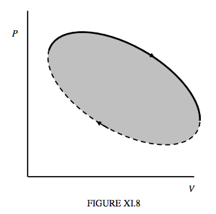
Figure XI.8 illustrates schematically the path taken by the state of a working substance is a generalized heat engine. In the upper part of the cycle (continuous curve) the working substance is expanding, and the machine is doing work. The work done by the engine is ∫PdV, or the area under that part of the curve. In the lower part of the cycle (dashed curve) the working substance is being compressed; work is being done on it. This work is the area under the dashed portion of the cycle. The net work done by the engine during the cycle is the work done by the engine while it is expanding minus the work done on it during the compression part of the cycle, and this is the area enclosed by the cycle.
During one part of any heat engine cycle, heat is supplied to the engine, and during other parts, heat is lost from it. As described in Section 11.1, the efficiency η of a heat engine is defined by
\[ \eta=\frac{\textbf{ net} ~ \text{external work done} ~ \textbf{by} ~ \text{the engine during a cycle}}{\text {heat supplied} ~ \textbf{to} ~ \textbf{the engine during a cycle.}}\]
Note that the word “net” does not appear in the denominator. The efficiency can also be calculated from
\[ \eta=\frac{Q_{\text { in }}-Q_{\text { out }}}{Q_{\text { in }}},\]
though I stress that this is not a definition.
In the Carnot engine, which is the most efficient conceivable engine for given source and sink temperature, the efficiency is
\[ \eta=\frac{T_{2}-T_{1}}{T_{2}},\]
where T2 and T1 are respectively the temperatures of the hot source and cold sink.
If the working substance is taken round a cycle in the PV-plane in the counterclockwise direction, the device is a refrigerator.
In that case the area enclosed by the cycle is equal to the net work that is done on the working substance. If the refrigerator operates on a reverse Carnot cycle, the working substance takes in (from whatever it is that it is trying to cool) a quantity of heat Q1 as it expands isothermally from d to c (see figure XI.1, but with the arrows reversed) and expels a (greater) quantity of heat Q2 as it is compressed isothermally from b to a. This quantity Q2 is expelled into the room – which is why the room gets warmer when you switch on the fridge. (What – you never noticed?) The refrigerating effect is Q1, since this is the quantity of heat taken in by the refrigerator from the body that is to be cooled.
The coefficient of performance of a refrigerator is defined by
\[ \frac{\text { refrigerating effect }}{\text { net work done} ~ \textbf{on} ~ \text{the engine during the cycle. }}\]
By the first law of thermodynamics, the denominator of the expression is Q2 − Q1, and for a reversible Carnot cycle, the entropy in equals the entropy out, so that Q2/Q1 = T2/T1. Therefore the coefficient of performance for a Carnot refrigeration cycle can be calculated from
\[ \frac{T_{1}}{T_{2}-T_{1}}.\]
This, of course, can be much greater than 1 – but no refrigerator working between the same source and sink temperatures can have a coefficient of performance greater that that of a reversible Carnot refrigerator.
Of course the working substance in a real refrigerator (“fridge”) is not an ideal gas, nor does one follow a Carnot cycle – there are too many practical difficulties in the way of achieving this ideal dream. As mentioned elsewhere in this course, I am not a practical man and I am not suited to describing real, practical machines. The fundamental principles described in this section do, of course, still apply in the real world! In a real refrigerator, the working substance (the refrigerant) is a volatile fluid which is vaporized in one part of the operation and condensed to a liquid in another part. In industrial refrigerators, the refrigerant may be ammonia, but this is considered to be too dangerous for domestic use. “Freon”, which was a mixture of chlorofluorocarbons, such as CCl2F2, was in fashion for a while, but escaping chlorofluorocarbons have been known for some time to cause breakdown of ozone (O3) in the atmosphere, thus destroying our protection against ultraviolet radiation from the Sun. The chlorofluorocarbons have been largely replaced by hydrofluorocarbons, such as C2H2F4, which are believed to be less damaging to the ozone layer. The exact formula or mixture is doubtless a trade secret.
The fluid is forced around a system of tubes by a pump called the compressor. Shortly before the fluid reaches the freezer it is in liquid form, moving along some rather narrow pipes. It is then forced through a nozzle into a system of wider pipes (the evaporator) surrounding the freezer, and there it vaporizes, taking heat from the food and from the air in the freezer. A fan may also distribute the cooled air throughout the rest of the refrigerator. After leaving the freezer, the vapour returns to the compressor, where it is, of course, compressed (which is why the pump is called the compressor). This produces heat, which is dissipated into the room as the fluid is forced through a series of pipes and vanes, known as the condenser, at the rear of the fridge, where the fluid condenses into liquid form again. The cycle then starts anew.
The following summary of Carnot heat engines and refrigerators may be helpful. (But just remember that, while Carnot cycles are the most efficient engines and refrigerators for given source and sink temperatures, the practical realization of a real engine or refrigerator may not be identical to this theoretical ideal.)
Notation:
T2 = hotter temperature
T1 = cooler temperature
Q2 = heat gained or lost at T2
Q1 = heat gained or lost at T1
\( \Delta S=0 \qquad \frac{Q_{1}}{T_{1}}=\frac{Q_{2}}{T_{2}}\)
Heat Engine:
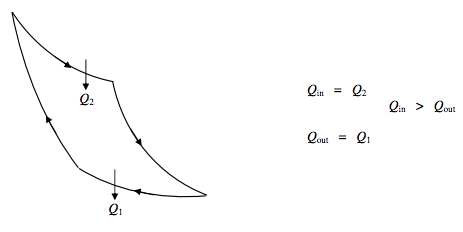
\(\Delta U=0 \quad \text { Net work done}~ \textbf{by} ~ \text{engine }=Q_{2}-Q_{1}.\)
\( \text { Efficiency } \eta=\frac{Q_{i n}-Q_{\text { out }}}{Q_{\text { in }}}=\frac{Q_{2}-Q_{1}}{Q_{2}}=\frac{T_{2}-T_{1}}{T_{2}}\)
Refrigerator:
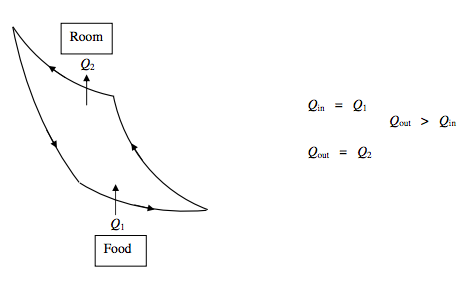
\(\Delta U=0 \qquad \text { Net work done} ~ \textbf{ on} ~ \text{refrigerator }=Q_{2}-Q_{1}\)
\( \text { Coefficient of Performance } P=\frac{Q_{\text { in }}}{Q_{\text { oxt }}-Q_{\text { in }}}=\frac{Q_{1}}{Q_{2}-Q_{1}}=\frac{T_{1}}{T_{2}-T_{1}}\)
Heat Pump:
The principle of a heat pump is the same as that of a refrigerator, except that its purpose is different. The purpose of a refrigerator is to extract heat from something (e.g. food) and so to make it colder. That the heat so extracted goes into the room to make the room warmer (at least in principle) is incidental. The important thing is how much heat is extracted from the food, and that is why it is appropriate to define the coefficient of performance of a refrigerator as the refrigerating effect (i.e. Q1) divided by the net work done on the refrigerator, per cycle. But with a heat pump, the object is to heat the room by extracting heat from outside. That the outside may become cooler (at least in principle) is incidental. Thus, for a heat pump, the appropriate definition of the coefficient of performance is the heating effect (i.e. Q2) divided by the net work done on the refrigerator, per cycle.
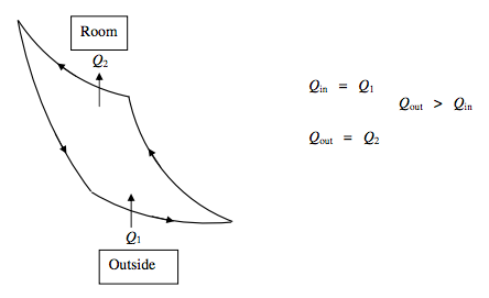
\( \Delta U=0 \qquad \text { Net work done} ~ \textbf{on} ~ \text{heat pump }=Q_{2}-Q_{1}\)
\( \text{Coefficient of Performance} ~ P=\frac{Q_{\mathrm{out}}}{Q_{\mathrm{out}}-Q_{\mathrm{in}}}=\frac{Q_{2}}{Q_{2}-Q_{1}}=\frac{T_{2}}{T_{2}-T_{1}}\)
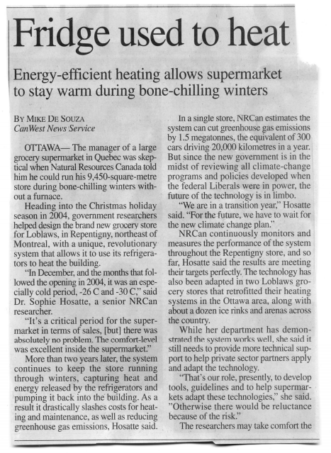
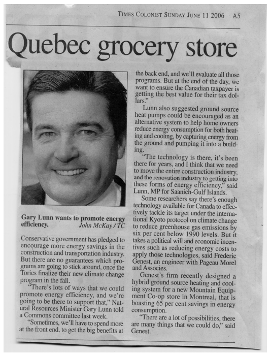
You can see from this equation that, the warmer it is outside (T1), the greater the coefficient of performance. You may therefore wonder if it is practical to use a heat pump to heat a building in a cold climate, such as the Quebec winter. And, if it isn’t, can one devise an engine that is simultaneously a refrigerator and a heat pump; that is to say, it extracts heats from (i.e. cools) the food, and transfers this heat (plus a little bit more because of the work that is done on the refrigerator/heat pump) into the room in order to heat the room effectively. There’s an answer to that in an article in the Victoria Times-Colonist of June 11, 2006, which I reproduce, with permission, below.
Air Conditioner
The purpose of a refrigerator (“fridge”) is to pump some heat Q1 from the food (or whatever is to be kept cool). The quantity Q1 is the “refrigerating effect”. During the operation of the fridge, a somewhat greater quantity Q2 of heat is expelled into the room, though this should not result in a very noticeable rise in temperature of the room, partly because the room has a large thermal capacity, and partly because much of this heat will be lost through the windows. The coefficient of performance of the fridge is the refrigerating effect per cycle, Q1, divided by the net work done on the fridge per cycle, and, for a Carnot cycle it can be calculated from T1/(T2 − T1).
The purpose of a heat pump is to pump some heat Q1 from outside, and (from the work done on the pump) to pump a larger quantity Q2 of heat into the room – large enough, indeed to warm the room appreciably, supposing that you don’t keep all the windows wide open. The coefficient of performance must therefore be defined as Q2 divided by the net work done on the fridge per cycle. For a Carnot cycle it can be calculated from T2/(T2 − T1).
There is a third possibility, namely an air conditioner. This will incorporate a dehumidifier, but, in our present context we regard it as a device whose purpose is to pump heat from the room to the outside, rather than from outside to the room. If it is successful, the room will become cooler than the outside. Thus an air conditioner is more like a refrigerator, in that the coefficient of performance is the heat Q1 extracted per cycle from the room divided by the net work done on the machine per cycle. For a Carnot cycle it can be calculated from T1/(T2 − T1).
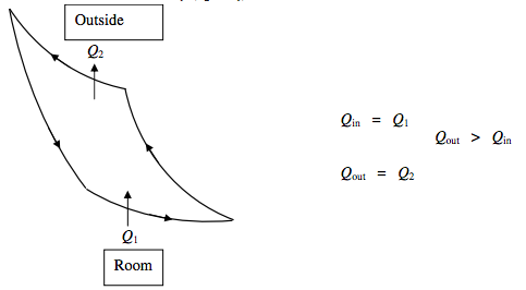
\( \Delta U=0 \qquad \text { Net work done} ~ \textbf{on} ~ \text{air conditioner }=Q_{2}-Q_{1}\).
\(\text { Coefficient of Performance } P=\frac{Q_{\text { in }}}{Q_{\text { out }}-Q_{\text { in }}}=\frac{Q_{1}}{Q_{2}-Q_{1}}=\frac{T_{1}}{T_{2}-T_{1}}\).
Those who have read thus far will have an idea that there are things called heat engines, refrigerators, heat pumps and air conditioners, which are represented by Carnot cycles or similar cycles, with arrows going in different directions, a few equations with different subscripts, and subtly different definitions of efficiency or coefficient of performance. Since I prepared these notes I have discovered that there actually exist in the real world, real, solid machines called heat engines, refrigerators, heat pumps and air conditioners. I have discovered two very nice little pamphlets describing real heat pumps and real air conditioners, and how you might install them to heat or to cool your home. They are called Heating and Cooling with a Heat Pump, and Air Conditioning your Home, each about 50 pages. My copies are dated 1996, revised 2004, though I dare say you might be able to get more recent ones. They are available free from Energy Publications, Office of Energy Efficiency, Natural Resources Canada, c/o S.J.D.S., 1779 Pink Road, Gatineau, Province of Québec, Canada J9J 3N7. I found them fascinating.


