9.2: Free Energy of the One-Dimensional Ising Model
- Page ID
- 6386
\( \newcommand{\vecs}[1]{\overset { \scriptstyle \rightharpoonup} {\mathbf{#1}} } \)
\( \newcommand{\vecd}[1]{\overset{-\!-\!\rightharpoonup}{\vphantom{a}\smash {#1}}} \)
\( \newcommand{\id}{\mathrm{id}}\) \( \newcommand{\Span}{\mathrm{span}}\)
( \newcommand{\kernel}{\mathrm{null}\,}\) \( \newcommand{\range}{\mathrm{range}\,}\)
\( \newcommand{\RealPart}{\mathrm{Re}}\) \( \newcommand{\ImaginaryPart}{\mathrm{Im}}\)
\( \newcommand{\Argument}{\mathrm{Arg}}\) \( \newcommand{\norm}[1]{\| #1 \|}\)
\( \newcommand{\inner}[2]{\langle #1, #2 \rangle}\)
\( \newcommand{\Span}{\mathrm{span}}\)
\( \newcommand{\id}{\mathrm{id}}\)
\( \newcommand{\Span}{\mathrm{span}}\)
\( \newcommand{\kernel}{\mathrm{null}\,}\)
\( \newcommand{\range}{\mathrm{range}\,}\)
\( \newcommand{\RealPart}{\mathrm{Re}}\)
\( \newcommand{\ImaginaryPart}{\mathrm{Im}}\)
\( \newcommand{\Argument}{\mathrm{Arg}}\)
\( \newcommand{\norm}[1]{\| #1 \|}\)
\( \newcommand{\inner}[2]{\langle #1, #2 \rangle}\)
\( \newcommand{\Span}{\mathrm{span}}\) \( \newcommand{\AA}{\unicode[.8,0]{x212B}}\)
\( \newcommand{\vectorA}[1]{\vec{#1}} % arrow\)
\( \newcommand{\vectorAt}[1]{\vec{\text{#1}}} % arrow\)
\( \newcommand{\vectorB}[1]{\overset { \scriptstyle \rightharpoonup} {\mathbf{#1}} } \)
\( \newcommand{\vectorC}[1]{\textbf{#1}} \)
\( \newcommand{\vectorD}[1]{\overrightarrow{#1}} \)
\( \newcommand{\vectorDt}[1]{\overrightarrow{\text{#1}}} \)
\( \newcommand{\vectE}[1]{\overset{-\!-\!\rightharpoonup}{\vphantom{a}\smash{\mathbf {#1}}}} \)
\( \newcommand{\vecs}[1]{\overset { \scriptstyle \rightharpoonup} {\mathbf{#1}} } \)
\( \newcommand{\vecd}[1]{\overset{-\!-\!\rightharpoonup}{\vphantom{a}\smash {#1}}} \)
\(\newcommand{\avec}{\mathbf a}\) \(\newcommand{\bvec}{\mathbf b}\) \(\newcommand{\cvec}{\mathbf c}\) \(\newcommand{\dvec}{\mathbf d}\) \(\newcommand{\dtil}{\widetilde{\mathbf d}}\) \(\newcommand{\evec}{\mathbf e}\) \(\newcommand{\fvec}{\mathbf f}\) \(\newcommand{\nvec}{\mathbf n}\) \(\newcommand{\pvec}{\mathbf p}\) \(\newcommand{\qvec}{\mathbf q}\) \(\newcommand{\svec}{\mathbf s}\) \(\newcommand{\tvec}{\mathbf t}\) \(\newcommand{\uvec}{\mathbf u}\) \(\newcommand{\vvec}{\mathbf v}\) \(\newcommand{\wvec}{\mathbf w}\) \(\newcommand{\xvec}{\mathbf x}\) \(\newcommand{\yvec}{\mathbf y}\) \(\newcommand{\zvec}{\mathbf z}\) \(\newcommand{\rvec}{\mathbf r}\) \(\newcommand{\mvec}{\mathbf m}\) \(\newcommand{\zerovec}{\mathbf 0}\) \(\newcommand{\onevec}{\mathbf 1}\) \(\newcommand{\real}{\mathbb R}\) \(\newcommand{\twovec}[2]{\left[\begin{array}{r}#1 \\ #2 \end{array}\right]}\) \(\newcommand{\ctwovec}[2]{\left[\begin{array}{c}#1 \\ #2 \end{array}\right]}\) \(\newcommand{\threevec}[3]{\left[\begin{array}{r}#1 \\ #2 \\ #3 \end{array}\right]}\) \(\newcommand{\cthreevec}[3]{\left[\begin{array}{c}#1 \\ #2 \\ #3 \end{array}\right]}\) \(\newcommand{\fourvec}[4]{\left[\begin{array}{r}#1 \\ #2 \\ #3 \\ #4 \end{array}\right]}\) \(\newcommand{\cfourvec}[4]{\left[\begin{array}{c}#1 \\ #2 \\ #3 \\ #4 \end{array}\right]}\) \(\newcommand{\fivevec}[5]{\left[\begin{array}{r}#1 \\ #2 \\ #3 \\ #4 \\ #5 \\ \end{array}\right]}\) \(\newcommand{\cfivevec}[5]{\left[\begin{array}{c}#1 \\ #2 \\ #3 \\ #4 \\ #5 \\ \end{array}\right]}\) \(\newcommand{\mattwo}[4]{\left[\begin{array}{rr}#1 \amp #2 \\ #3 \amp #4 \\ \end{array}\right]}\) \(\newcommand{\laspan}[1]{\text{Span}\{#1\}}\) \(\newcommand{\bcal}{\cal B}\) \(\newcommand{\ccal}{\cal C}\) \(\newcommand{\scal}{\cal S}\) \(\newcommand{\wcal}{\cal W}\) \(\newcommand{\ecal}{\cal E}\) \(\newcommand{\coords}[2]{\left\{#1\right\}_{#2}}\) \(\newcommand{\gray}[1]{\color{gray}{#1}}\) \(\newcommand{\lgray}[1]{\color{lightgray}{#1}}\) \(\newcommand{\rank}{\operatorname{rank}}\) \(\newcommand{\row}{\text{Row}}\) \(\newcommand{\col}{\text{Col}}\) \(\renewcommand{\row}{\text{Row}}\) \(\newcommand{\nul}{\text{Nul}}\) \(\newcommand{\var}{\text{Var}}\) \(\newcommand{\corr}{\text{corr}}\) \(\newcommand{\len}[1]{\left|#1\right|}\) \(\newcommand{\bbar}{\overline{\bvec}}\) \(\newcommand{\bhat}{\widehat{\bvec}}\) \(\newcommand{\bperp}{\bvec^\perp}\) \(\newcommand{\xhat}{\widehat{\xvec}}\) \(\newcommand{\vhat}{\widehat{\vvec}}\) \(\newcommand{\uhat}{\widehat{\uvec}}\) \(\newcommand{\what}{\widehat{\wvec}}\) \(\newcommand{\Sighat}{\widehat{\Sigma}}\) \(\newcommand{\lt}{<}\) \(\newcommand{\gt}{>}\) \(\newcommand{\amp}{&}\) \(\definecolor{fillinmathshade}{gray}{0.9}\)The N-spin one-dimensional Ising model consists of a horizontal chain of spins, s1, s2, . . . , sN, where si = ±1.

A vertical magnetic field H is applied, and only nearest neighbor spins interact, so the Hamiltonian is
\[ \mathcal{H}_{N}=-J \sum_{i=1}^{N-1} s_{i} s_{i+1}-m H \sum_{i=1}^{N} s_{i}.\]
For this system the partition function is
\[ Z_{N}=\sum_{\text { states }} e^{-\beta \mathcal{H}_{N}}=\sum_{s_{1}=\pm 1} \sum_{s_{2}=\pm 1} \cdots \sum_{s_{N}=\pm 1} e^{K \sum_{i=1}^{N-1} s_{i} s_{i+1}+L \sum_{i=1}^{N} s_{i}},\]
where
\[ K \equiv \frac{J}{k_{B} T} \quad \text { and } \quad L \equiv \frac{m H}{k_{B} T}.\]
If J = 0, (the ideal paramagnet) the partition function factorizes, and the problem is easily solved using the “summing Hamiltonian yields factorizing partition function” theorem. If H = 0, the partition function nearly factorizes, and the problem is not too difficult. (See problem 9.3.) But in general, there is no factorization.
We will solve the problem using induction on the size of the system. If we add one more spin (spin number N + 1), then the change in the system’s energy depends only upon the state of the new spin and of the previous spin (spin number N). Define Z↑N as, not the sum over all states, but the sum over all states in which the last (i.e. Nth) spin is up, and define Z↓N as the sum over all states in which the last spin is down, so that
\[ Z_{N}=Z_{N}^{\uparrow}+Z_{N}^{\downarrow}.\]
Now, if one more spin is added, the extra term in e−βH results in a factor of
\[ e^{K s_{N} s_{N+1}+L s_{N+1}}.\]
From this, it is very easy to see that
\[ Z_{N+1}^{\uparrow}=Z_{N}^{\uparrow} e^{K+L}+Z_{N}^{\downarrow} e^{-K+L}\]
\[ Z_{N+1}^{\downarrow}=Z_{N}^{\uparrow} e^{-K-L}+Z_{N}^{\downarrow} e^{K-L}.\]
This is really the end of the physics of this derivation. The rest is mathematics.
So put on your mathematical hats and look at the pair of equations above. What do you see? A matrix equation!
\[ \left(\begin{array}{c}{Z_{N+1}^{\uparrow}} \\ {Z_{N+1}^{\downarrow}}\end{array}\right)=\left(\begin{array}{cc}{e^{K+L}} & {e^{-K+L}} \\ {e^{-K-L}} & {e^{K-L}}\end{array}\right)\left(\begin{array}{c}{Z_{N}^{\uparrow}} \\ {Z_{N}^{\downarrow}}\end{array}\right).\]
We introduce the notation
\[ \mathbf{w}_{N+1}=\mathbf{T} \mathbf{w}_{N}\]
for the matrix equation. The 2 × 2 matrix T, which acts to add one more spin to the chain, is called the transfer matrix. Of course, the entire chain can be built by applying T repeatedly to an initial chain of one site, i.e. that
\[ \mathbf{w}_{N+1}=\mathbf{T}^{N} \mathbf{w}_{1},\]
where
\[ \mathbf{w}_{1}=\left(\begin{array}{c}{e^{L}} \\ {e^{-L}}\end{array}\right).\]
The fact that we are raising a matrix to a power suggests that we should diagonalize it. The transfer matrix T has eigenvalues λA and λB (labeled so that |λA| > |λB|) and corresponding eigenvectors xA and xB. Like any other vector, w1 can be expanded in terms of the eigenvectors
\[ \mathbf{w}_{1}=c_{A} \mathbf{x}_{A}+c_{B} \mathbf{x}_{B}\]
and in this form it is very easy to see what happens when w1 is multiplied by T N times:
\( \mathbf{w}_{N+1}=\mathbf{T}^{N} \mathbf{w}_{1}=c_{A} \top^{N} \mathbf{x}_{A}+c_{B} \mathbf{T}^{N} \mathbf{x}_{B}\)
\[ =c_{A} \lambda_{A}^{N} \mathbf{x}_{A}+c_{B} \lambda_{B}^{N} \mathbf{x}_{B}.\]
So the partition function is
\[ Z_{N+1}=Z_{N+1}^{\uparrow}+Z_{N+1}^{\downarrow}=c_{A} \lambda_{A}^{N}\left(x_{A}^{\uparrow}+x_{A}^{\downarrow}\right)+c_{B} \lambda_{B}^{N}\left(x_{B}^{\uparrow}+x_{B}^{\downarrow}\right).\]
By diagonalizing matrix T (that is, by finding both its eigenvalues and its eigenvectors) we could find every element in the right hand side of the above equation, and hence we could find the partition function ZN for any N. But of course we are really interested only in the thermodynamic limit N → ∞. Because |λA| > |λB|, λNA dominates λNB in the thermodynamic limit, and
\[ Z_{N+1} \approx c_{A} \lambda_{A}^{N}\left(x_{A}^{\uparrow}+x_{A}^{\downarrow}\right)\]
provided that \( c_{A}\left(x_{A}^{\uparrow}+x_{A}^{\downarrow}\right) \neq 0\). Now,
\[ F_{N+1}=-k_{B} T \ln Z_{N+1} \approx-k_{B} T N \ln \lambda_{A}-k_{B} T \ln \left[c_{A}\left(x_{A}^{\uparrow}+x_{A}^{\downarrow}\right)\right],\]
and this approximation becomes exact in the thermodynamic limit. Thus the free energy per spin is
\[ f(K, L)=\lim _{N \rightarrow \infty} \frac{F_{N+1}(K, L)}{N+1}=-k_{B} T \ln \lambda_{A}.\]
So to find the free energy we only need to find the larger eigenvalue of T: we don’t need to find the smaller eigenvalue, and we don’t need to find the eigenvectors!
It is a simple matter to find the eigenvalues of our transfer matrix T. They are the two roots of
\[ \operatorname{det}\left(\begin{array}{cc}{e^{K+L}-\lambda} & {e^{-K+L}} \\ {e^{-K-L}} & {e^{K-L}-\lambda}\end{array}\right)=0\]
\[ \left(\lambda-e^{K+L}\right)\left(\lambda-e^{K-L}\right)-e^{-2 K}=0\]
\[ \lambda^{2}-2 e^{K} \cosh L \lambda+e^{2 K}-e^{-2 K}=0,\]
which are
\[ \lambda=e^{K}\left[\cosh L \pm \sqrt{\cosh ^{2} L-1+e^{-4 K}}\right].\]
It is clear that both eigenvalues are real, and that the larger one is positive, so
\[ \lambda_{A}=e^{K}\left[\cosh L+\sqrt{\sinh ^{2} L+e^{-4 K}}\right].\]
Finally, using equation (9.17), we find the free energy per spin
\[ f(T, H)=-J-k_{B} T \ln \left[\cosh \frac{m H}{k_{B} T}+\sqrt{\sinh ^{2} \frac{m H}{k_{B} T}+e^{-4 J / k_{B} T}}\right].\]
Results
Knowing the free energy, we can take derivatives to find any thermodynamic quantity (see problem 9.2). Here I’ll sketch and discuss the results obtained through those derivatives.
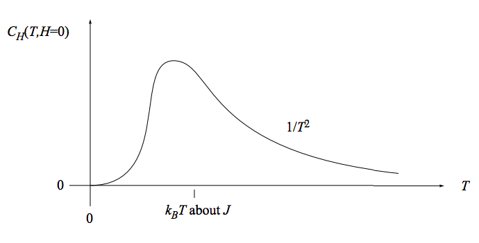
The heat capacity at constant, vanishing, magnetic field is sketched here:

Do you think an experimentalist needs a magnet to probe magnetic phenomena? This graph shows that a magnet is not required: The magnetic effects result in a bump in the heat capacity near kBT = J, even when no magnetic field is applied.
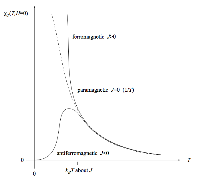
The magnetic susceptibility is sketched here:

We have already seen that for independent spins (paramagnet, J = 0) the susceptibility falls like 1/T with temperature (the “Curie law”). Interacting spins at high temperature \((k_B T \gg J)\) behave approximately the same way. But at low temperatures, the susceptibility for a ferromagnet exceeds the susceptibility for a paramagnet, while the susceptibility for a antiferromagnet undershoots the susceptibility for a paramagnet. This makes sense: For a paramagnet, the external magnetic field is inducing the spins to align. For a ferromagnet, both the external magnetic field and the tendency of neighboring spins to align are inducing the spins to align. For an antiferromagnet, the external magnetic field is inducing the spins to align, but the tendency of neighboring spins to antialign is opposing that inducement.
Aligning the spins in a paramagnet is like herding cats: the individual spins are independent and don’t naturally take to pointing all in the same direction. Aligning the spins in a ferromagnet is like herding cows: the individual spins want to all go in the same direction and don’t care which direction it is. Aligning the spins in an antiferromagnet is like herding siblings in a dysfunctional family, where each sibling says “I want to go to the opposite of wherever my brother/sister wants to go.”


