
3.1: Motion with Constant Speed


- Last updated
- Mar 28, 2024
- Save as PDF
( \newcommand{\kernel}{\mathrm{null}\,}\)
Now suppose that the ball in Figure 3.1.1 is rolling, and that we recorded its x position every second in a table and obtained the values in Table 3.1.1 (we will ignore measurement uncertainties and pretend that the values are exact).
| Time [s] | X position [m] |
|---|---|
| 0.0 s | 0.5 m |
| 1.0 s | 1.0 m |
| 2.0 s | 1.5 m |
| 3.0 s | 2.0 m |
| 4.0 s | 2.5 m |
| 5.0 s | 3.0 m |
| 6.0 s | 3.5 m |
| 7.0 s | 4.0 m |
| 8.0 s | 4.5 m |
| 9.0 s | 5.0 m |
Table 3.1.1: Position of a ball along the x-axis recorded every second.
The easiest way to visualize the values in the table is to plot them on a graph, as in Figure 3.1.1. Plotting position as a function of time is one of the most common graphs to make in physics, since it is often a complete description of the motion of an object. We can easily plot these values in Python:
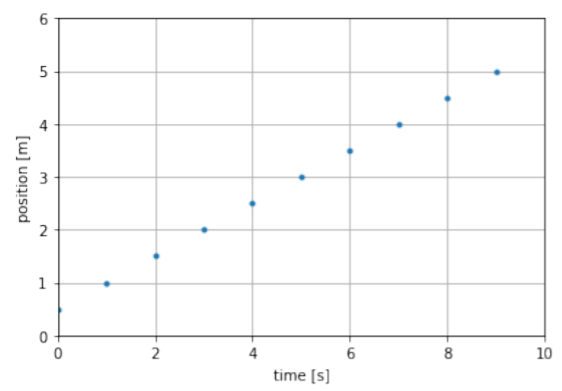
The data plotted in Figure 3.1.1 show that the x position of the ball increases linearly with time (i.e. it is a straight line). This means that in equal time increments, the ball will cover equal distances. Note that we also had the liberty to choose when we define t=0; in this case, we chose that time is zero when the ball is at x=0.5m.
Using the data from Table 3.1.1, at what position along the x-axis will the ball be when time is t=9.5 s, if it continues its motion undisturbed?
- 5.0m
- 5.25m
- 5.75m
- 6.0m
- Answer
- B. The ball is moving 0.5m each second. Therefore, in 0.5s it moves 0.25m and will be at position x=5.25m.
Since the position as a function of time for the ball plotted in Figure 3.1.1 is linear, we can summarize our description of the motion using a function, x(t), instead of having to tabulate the values as we did in Table 3.1.1. The function will have the functional form:
x(t)=x0+vxt
The constant x0 is the “offset” of the function, the value that the function has at t=0s. We call x0 the “initial position” of the object (its position at t=0). The constant vx is the “slope” of the function and gives the rate of change of the position as a function of time. We call vx the “velocity” of the object.
The initial position is simply the value of the position at t=0, and is given from the table as:
x0=0.5m
The velocity, vx, is simply the difference in position, ∆x, between any two points divided by the amount of time, ∆t, that it took the object to move between those to points (“rise over run” for the graph of x(t)):
v=∆x∆t
By looking at any two rows from Table 3.1.1, we can see that the object travels a distance ∆x=0.5m in a time ∆t=1s. Its velocity is thus:
v=ΔxΔt=(0.5m)(1s)=0.5m/s
The position of the object as a function of time is thus
x(t)=(0.5m)+(0.5m/s)t
If vx is large, then the object covers more distance in a given time, i.e. it moves faster. If vx is a negative number, then the object moves in the negative x direction. The speed of the object is the absolute value of its velocity. Thus objects moving in different directions will have different velocities, but can have the same speed if they cover the same amount of distance in the same amount of time.
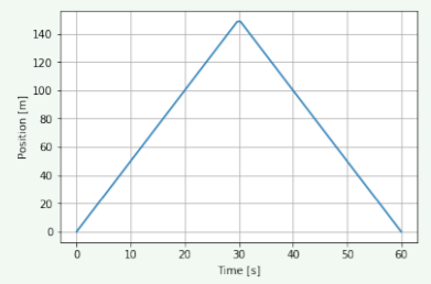
Referring to Figure 3.1.2, what can you say about the motion of the object?
- The object moved faster and faster between t=0s and t=30s, then slowed down to a stop at t=60s.
- The object moved in the positive x-direction between t=0s and t=30s, and then turned around and moved in the negative x-direction between t=30s and t=60s.
- The object moved faster between t=0s and t=30s than it did between t=30s and t=60s.
- Answer
- B. The object is moving at constant speed due to the straight line (uniform) motion. When the slope changes from positive to negative, the direction of the motion changes, but the slope remains the same magnitude.
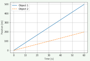
Referring to Figure 3.1.3, what can you say about the motion of the two objects?
- Object 1 is slower than Object 2
- Object 1 is more than twice as fast as Object 2
- Object 1 is less than twice as fast as Object 2
- Answer
- B. The distance traveled in 60s is 500m for Object 1 and 200m for Object 2. Therefore, Object 1 must be going more than twice as fast as Object 2. One could also note the slope of the graphs is 5:2 in ratio.