
5.5: Applying Newton’s Laws


- Last updated
- Mar 28, 2024
- Save as PDF
( \newcommand{\kernel}{\mathrm{null}\,}\)
Now that we have introduced all of the concepts from Newton’s Theory of Classical Physics, we present some general strategies for building models that use the theory. Recall that if we can describe the motion of all objects of interest to us, we have described everything that we can. Newton’s Second Law allows us to determine the acceleration of an object based on the net force acting on the object. Once we have determined the accelerations of all objects of interest we have built a complete model.
The most important step in applying Newton’s Theory is to identify the forces that are exerted on an object. The most important step in applying Newton’s Theory is to identify the forces that are exerted on an object. The most important step in applying Newton’s Theory is to identify the forces that are exerted on an object. Now that you have read it three times, you realize this step is important, right?!
The strategy for building a model for the motion of an object using Newton’s Theory is straightforward:
- Identify an inertial frame of reference in which to build the model.
- Identify the forces acting on the object (did we mention that this step is important?).
- Draw a free-body diagram.
- Apply Newton’s Second Law.
Identifying the forces
The first step in applying Newton’s theory is to identify all of the forces that are acting on an object. This can be done by asking yourself: “what could possibly be pushing or pulling on the object?”, as well as running through the list of forces that we enumerated in Section 5.2 to identify if any of them are relevant here. For easy reference, we reproduce the types of forces here and include some questions that you might ask yourself to decide whether or not to include the corresponding force:
- Weight (is the object near the surface of a planet?).
- Normal forces (is the object in contact with any surface? There could be more than one!).
- Frictional forces (are there static or kinetic friction forces associated with the normal forces?).
- Tension forces (is something like a rope pulling on the object?).
- Drag forces (is the object moving through a fluid?).
- Spring forces (is there a spring pushing or pulling on the object?).
- Applied forces (is anything else pushing or pulling on the object?).
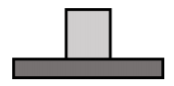
A block of mass m is at rest on a horizontal table, as shown in Figure 5.5.1. What forces are exerted on the block?
Solution
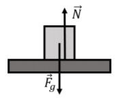
The forces on the block are illustrated in Figure 5.5.2 and are:
- →Fg, its weight.
- →N, a normal force exerted by the plane. The normal force is perpendicular to the interface between the table and the block. It points upwards in “reaction” to the downwards force that the block exerts onto the table. The downwards force from the block onto the table is not shown, since that force is not exerted on the block but on the table.
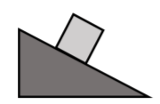
A block of mass m is at rest on a inclined surface, as shown in Figure 5.4.3. What forces are exerted on the block?
Solution
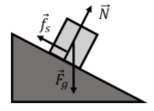
The forces on the block are illustrated in Figure 5.5.4 and are:
- →Fg, its weight.
- →N, a normal force exerted by the inclined plane.
- →fs, a force of static friction exerted by the inclined plane. Without this force, the block would slide down. The force is in the direction opposite of impeding motion and is parallel to the interface (and perpendicular to the normal force).
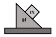
A block of mass m is at rest on a wedge-shaped block of mass M itself at rest on a horizontal table, as shown in Figure 5.5.5. What forces are exerted on each of the two blocks?
Solution
Since it will be too messy to draw all of the forces on the same diagram, we have drawn each block separately in Figure 5.5.5. Usually, when multiple blocks are stacked on each other, it is easiest to start with the forces on the top block. In this case, the top block is in the same condition as the block from Example 5.4.2. The forces exerted on the top block are:
- →Fmg, its weight.
- →Nm, a normal force from the wedge-shaped block.
- →fms, a force of static friction exerted by the wedge-shaped block.
The forces exerted on the wedge-shaped block are:
- →FMg, its weight.
- →NM, a normal force exerted by the small block. Note that this force is equal in magnitude and opposite in direction to →Nm (the two forces, →Nm and →NM, which are on different objects, are an action/reaction pair of forces).
- →fMs, a force of friction exerted by the small block (again, this forms an action/reaction pair of forces with →fms).
- NM2, a normal force exerted by the table.
The forces for both blocks are shown in Figure 5.5.6.
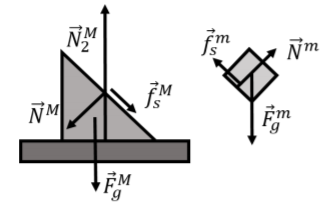
Free body diagrams
In order to analyze the forces on an object more clearly, it is a very good idea to draw a “Free-Body Diagram” (FBD). A free-body diagram is simply a diagram where we draw the forces on a single object and represent the object as a point. Because the object is a point, we do not worry where on the object the forces are exerted. In later chapters, we will see that for extended bodies, it does matter where the forces are applied. However, Newton’s Laws as presented so far are only valid for objects that can be represented as a small point.
In Example 5.4.3 above, we would draw one free-body diagram for each object (each mass), as shown in Figure 5.5.7.
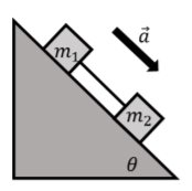
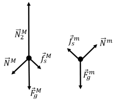
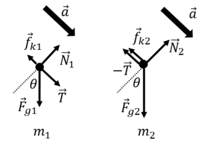
Two blocks, of masses m1 and m2, are placed on an inclined plane that makes an angle θ with the horizontal. The blocks are connected by a massless string, as shown in Figure 5.5.8. The two blocks are sliding and accelerating downwards with an acceleration, →a, as shown. The coefficient of kinetic friction between the plane and either block is µ_{k}. Draw a free-body diagram for each block.
Solution
First, we identify the forces on each mass (each block), which we then use to make the free-body diagram shown in Figure \PageIndex{8}. On mass m_1, the forces are:
- \vec F_{g1}, its weight.
- \vec N_1, a normal force exerted by the inclined plane.
- \vec f_{k1}, a force of kinetic friction exerted by the inclined plane. The force is in the opposite direction of the motion, and has a magnitude given by f_{k1}=\mu_kN_1.
- \vec T, a force of tension from the string.
On mass m_2, the forces are:
- \vec F_{g2}, its weight.
- \vec N_2, a normal force from the inclined plane.
- \vec f_{k2}, a force of kinetic friction exerted by the inclined plane. The force is in the opposite direction of the motion, and has a magnitude given by f_{k2}=\mu_kN_2.
- -\vec T, a force of tension from the string. This is the same force as on m_1, but in the opposite direction. We chose to label the force as -\vec T, instead of using a different variable, since it is just the negative of the vector that represents the tension force on m_1.
In Figure \PageIndex{9}, we have shown the forces on each block using a free-body diagram. We also reproduced the vector for the acceleration (we drew the vector for the acceleration using a thicker arrow to indicate that it has a different dimension). We also reproduced the angle \theta in the free-body diagram, as this is helpful once the free-body diagram is used with Newton’s Second Law.
Using Newton’s Second Law
Applying Newton’s Second Law is straightforward once all of the forces exerted on an object have been identified. You should thus make sure that you spend most of your time drawing a good and complete free-body diagram before proceeding.
Newton’s Second Law is a vector equation that relates the vector sum of all forces exerted on an object and the acceleration vector of the object. This corresponds to one scalar equation per component of the vector.
\begin{aligned} \sum \vec F &=m\vec a\\[4pt] \sum F_x &= ma_x \\[4pt] \sum F_y &= ma_y \\[4pt] \sum F_z &= ma_z\end{aligned}
In order to use Newton’s Second Law, we thus need to introduce a coordinate system so that we can work with the components of the vectors (forces and acceleration) in that coordinate system. Usually, a good choice of coordinate system is one where the x (or y) axis is parallel to the acceleration vector. Figure \PageIndex{10} shows the free-body diagram from the m_1 block from the previous example (Example 5.4.4) along with a good choice of coordinate system.
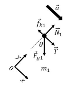
To apply Newton’s Second Law using the free-body diagram and coordinate system from Figure \PageIndex{10}, we first write out all of the vector and then identify their x and y components. The force vectors are:
\begin{aligned} \vec T &= T\hat x+0\hat y\\[4pt] \vec f_{k1}&=-f_{k1}\hat x+0\hat y\\[4pt] \vec F_{g1}&=m_1g(\sin\theta \hat x-\cos\theta \hat y)\\[4pt] \vec N_1&=0\hat x+N_1\hat y\end{aligned}
We can now write out the x component of Newton’s Second Law:
\begin{aligned} \sum F_x = T-f_{k1}-F_{g1}\sin\theta &= m_1 a\\[4pt] \therefore T-f_{k1}-F_{g1}\sin\theta &= m_1 a\end{aligned}
where we note that the normal force has no component in the x direction. The y component of Newton’s Second Law for mass m_1 is given by:
\begin{aligned} \sum F_y = N_1-F_{g1}&=0\\[4pt] \therefore N_1-F_{g1}&=0\end{aligned}
where we note that the forces of tension and friction have no y component. The two equations that we obtained above for x and y fully specify the motion of the m_1 block if all quantities are known3.
A few notes on applying Newton’s Second Law:
- When applying Newton’s Second Law, analyze each mass in the problem separately. It does not matter that block m_1 is connected by a rope to block m_2. Once you have determined all of the forces exerted on m_1, you can write Newton’s Second Law for m_1.
- Newton’s Second Law is a vector equation; this means that it is true for each (scalar) component of the vectors involved.
- You can choose the coordinate system, so choose one that makes it easy to write out the vector components. A good choice is to choose x to be parallel to the acceleration vector, so that you do not have to break the acceleration vector up into components. The choice of coordinate system is only made in order to allow you to write out the components of Newton’s Second Law based on the free-body diagram.
- Treat each mass separately (since Newton’s Second Law is only true for an individual mass). This means that each mass will have its own free-body diagram and that you can choose the coordinate system that is most convenient for a given free-body diagram. In particular, this means that you do not need to choose the same coordinate system for different masses in a problem.
The following example shows how to write Newton’s Second Law for a system of two blocks.
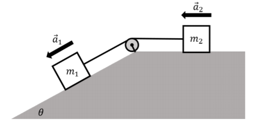
A block of mass m_1 is placed on an incline that makes an angle of \theta with the horizontal. The block of mass m_1 is connected by a massless string through a massless pulley to a second block of mass m_2, which rests on a horizontal surface. The blocks are accelerating in such a way that the block of mass m_1 is accelerating down the incline, as shown in Figure \PageIndex{5}. The coefficient of kinetic friction between either block and the surface it is resting on is \mu_k. Write Newton’s Second Law for both blocks.
Solution
First, we identify the forces on each mass (each block). On mass m_1, the forces are:
- \vec F_{g1}, its weight.
- \vec N_1, a normal force exerted by the inclined plane.
- \vec f_{k1}, a force of kinetic friction exerted by the inclined plane. The force is in the opposite direction of the motion, and has a magnitude given by f_{k1}=\mu_kN_1.
- \vec T_1, a force of tension from the string.
On mass m_2, the forces are:
- \vec F_{g2}, its weight.
- \vec N_2, a normal force from the horizontal surface.
- \vec f_{k2}, a force of kinetic friction exerted by the horizontal surface. The force is in the opposite direction of the motion, and has a magnitude given by f_{k2}=\mu_kN_2.
- \vec T_2, a force of tension from the string. This force has the same magnitude as the tension force \vec T_1 exerted on mass m_1, because the pulley is massless.
We can then proceed to draw the free-body diagram for each mass, and use that to write out Newton’s Second Law. For mass m_1, the free-body diagram is shown in Figure \PageIndex{12}. We have chosen a coordinate system that has the x axis parallel to the acceleration of the block, and the y axis upwards and perpendicular to the x axis, as shown.
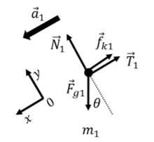
For m_1, we can write Newton’s Second Law, starting with the x components:
\begin{aligned} \sum F_x = F_{g1}\sin\theta-f_{k1}-T_1&=m_1a_1\\[4pt] \therefore m_1 g\sin\theta -\mu_k N_1 - T_1 &= m_1 a_1\end{aligned}
where, in the second line, we used the magnitude of the weight (F_{g1}=m_1g) and of the force of kinetic friction (f_{k1}=\mu_kN_1). For the y component of Newton’s Second Law, in which the acceleration has no component, we have:
\begin{aligned} \sum F_y = N_1 - F_{g1}\cos\theta &= 0\\[4pt] \therefore N_1=m_1g\cos\theta\end{aligned}
which shows us that the magnitude of the normal force can easily be expressed in terms of the weight (F_{g1}=m_1g) and the angle of the incline.
For m_2, we can proceed in much the same way, choosing a different coordinate system, since the acceleration vector for m_2 points in a different direction (we don’t have to choose a different coordinate system, but we can if we find it makes things easier). The free-body diagram for m_2 is shown in Figure \PageIndex{13} along with our choice of coordinate system.
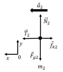
We start by writing out the x component of Newton’s Second Law for m_2:
\begin{aligned} \sum F_x = T_2 - f_{k2} &= m_2 a_2\\[4pt] \therefore T_2 - \mu_k N_2 = m_2 a_2\end{aligned}
where again, we expressed the kinetic force of friction using the normal force and the coefficient of kinetic friction. The y component of Newton’s Second Law gives:
\begin{aligned} \sum F_y = F_{g2}-N_2 &=0\\[4pt] \therefore N_2 = m_2g\end{aligned}
where again, we expressed the weight in terms of the mass and g, and we find that the normal force has the same magnitude as the weight.
Now that we have written Newton’s Second Law for each mass, we can write all four equations that we obtained to describe the system of two masses. We should also note that the magnitude of the tension forces are the same for the two masses (T_1=T_2=T), and that since the masses are connected by a string, the magnitude of their acceleration vectors are the same (a_1=a_2=a). Using this, we can describe the full system with the following 4 equations:
\begin{aligned} m_1 g\sin\theta -\mu_k N_1 - T &= m_1 a\\[4pt] N_1=m_1g\cos\theta\\[4pt] T - \mu_k N_2 = m_2 a\\[4pt] N_2 = m_2g\end{aligned}
Of the variables above (m_1, m_2, \mu_k, T, N_1, N_2, a), one would only need to specify all but four of them to fully describe the motion of the system. For example, if one specifies the two masses and the coefficient of kinetic friction, all of the other variables can be determined.
Footnotes
3. Since we have two equations, we technically only need to specify all but two quantities to be able to fully model the motion of the block.