26.1: Functions of Real Numbers

Last updated
Save as PDF

Page ID: 19571

\( \newcommand{\vecs}[1]{\overset { \scriptstyle \rightharpoonup} {\mathbf{#1}} } \) \( \newcommand{\vecd}[1]{\overset{-\!-\!\rightharpoonup}{\vphantom{a}\smash {#1}}} \)\(\newcommand{\id}{\mathrm{id}}\) \( \newcommand{\Span}{\mathrm{span}}\) \( \newcommand{\kernel}{\mathrm{null}\,}\) \( \newcommand{\range}{\mathrm{range}\,}\) \( \newcommand{\RealPart}{\mathrm{Re}}\) \( \newcommand{\ImaginaryPart}{\mathrm{Im}}\) \( \newcommand{\Argument}{\mathrm{Arg}}\) \( \newcommand{\norm}[1]{\| #1 \|}\) \( \newcommand{\inner}[2]{\langle #1, #2 \rangle}\) \( \newcommand{\Span}{\mathrm{span}}\) \(\newcommand{\id}{\mathrm{id}}\) \( \newcommand{\Span}{\mathrm{span}}\) \( \newcommand{\kernel}{\mathrm{null}\,}\) \( \newcommand{\range}{\mathrm{range}\,}\) \( \newcommand{\RealPart}{\mathrm{Re}}\) \( \newcommand{\ImaginaryPart}{\mathrm{Im}}\) \( \newcommand{\Argument}{\mathrm{Arg}}\) \( \newcommand{\norm}[1]{\| #1 \|}\) \( \newcommand{\inner}[2]{\langle #1, #2 \rangle}\) \( \newcommand{\Span}{\mathrm{span}}\)\(\newcommand{\AA}{\unicode[.8,0]{x212B}}\)

In calculus, we work with functions and their properties, rather than with variables as we do in algebra. We are usually concerned with describing functions in terms of their slope, the area (or volumes) that they enclose, their curvature, their roots (when they have a value of zero) and their continuity. The functions that we will examine are a mapping from one or more independent real numbers to one real number. By convention, we will use \(x,y,z\) to indicate independent variables, and \(f()\) and \(g()\), to denote functions. For example, if we say:

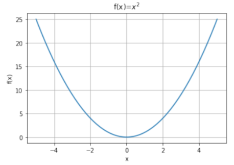
\[\begin{aligned} f(x) &= x^2\\[4pt] \therefore f(2) &= 4\end{aligned}\]

we mean that \(f(x)\) is a function that can be evaluated for any real number, \(x\), and the result of evaluating the function is to square the number \(x\). In the second line, we evaluated the function with \(x=2\). Similarly, we can have a function, \(g(x,y)\) of multiple variables:

\[\begin{aligned} g(x,y)&=x^2+2y^2\\[4pt] \therefore g(2,3)&=22\end{aligned}\]

We can easily visualize a function of 1 variable by plotting it, as in Figure A2.1.1.

Figure A2.1.1: \(f(x)=x^{2}\) plotted between \(x=-5\) and \(x=+5\).

Plotting a function of 2 variables is a little trickier, since we need to do it in three dimensions (one axis for \(x\), one axis for \(y\), and one axis for \(g(x,y)\)). Figure A2.1.2 shows an example of plotting a function of 2 variables.

Figure A2.1.2: \(g(x, y) = x^{2} + 2y^{2}\) plotted for \(x\) between \(-5\) and \(+5\) and for \(y\) between \(-5\) and \(+5\). A function of two variables can be visualized as a surface in three dimensions. One can also visualize the function by look at its “contours” (the lines drawn in the \(xy\) plane).

Unfortunately, it becomes difficult to visualize functions of more than 2 variables, although one can usually look at projections of those functions to try and visualize some of the features (for example, contour maps are 2D projections of 3D surfaces, as shown in the \(xy\) plane of Figure A1.1.2). When you encounter a function, it is good practice to try and visualize it if you can. For example, ask yourself the following questions:

Does the function have one or more maxima and/or minima?
Does the function cross zero?
Is the function continuous everywhere?
Is the function always defined for any value of the independent variables?