
26.3: Anti-derivatives and integrals
- Page ID
- 19573

\( \newcommand{\vecs}[1]{\overset { \scriptstyle \rightharpoonup} {\mathbf{#1}} } \)
\( \newcommand{\vecd}[1]{\overset{-\!-\!\rightharpoonup}{\vphantom{a}\smash {#1}}} \)
\( \newcommand{\dsum}{\displaystyle\sum\limits} \)
\( \newcommand{\dint}{\displaystyle\int\limits} \)
\( \newcommand{\dlim}{\displaystyle\lim\limits} \)
\( \newcommand{\id}{\mathrm{id}}\) \( \newcommand{\Span}{\mathrm{span}}\)
( \newcommand{\kernel}{\mathrm{null}\,}\) \( \newcommand{\range}{\mathrm{range}\,}\)
\( \newcommand{\RealPart}{\mathrm{Re}}\) \( \newcommand{\ImaginaryPart}{\mathrm{Im}}\)
\( \newcommand{\Argument}{\mathrm{Arg}}\) \( \newcommand{\norm}[1]{\| #1 \|}\)
\( \newcommand{\inner}[2]{\langle #1, #2 \rangle}\)
\( \newcommand{\Span}{\mathrm{span}}\)
\( \newcommand{\id}{\mathrm{id}}\)
\( \newcommand{\Span}{\mathrm{span}}\)
\( \newcommand{\kernel}{\mathrm{null}\,}\)
\( \newcommand{\range}{\mathrm{range}\,}\)
\( \newcommand{\RealPart}{\mathrm{Re}}\)
\( \newcommand{\ImaginaryPart}{\mathrm{Im}}\)
\( \newcommand{\Argument}{\mathrm{Arg}}\)
\( \newcommand{\norm}[1]{\| #1 \|}\)
\( \newcommand{\inner}[2]{\langle #1, #2 \rangle}\)
\( \newcommand{\Span}{\mathrm{span}}\) \( \newcommand{\AA}{\unicode[.8,0]{x212B}}\)
\( \newcommand{\vectorA}[1]{\vec{#1}} % arrow\)
\( \newcommand{\vectorAt}[1]{\vec{\text{#1}}} % arrow\)
\( \newcommand{\vectorB}[1]{\overset { \scriptstyle \rightharpoonup} {\mathbf{#1}} } \)
\( \newcommand{\vectorC}[1]{\textbf{#1}} \)
\( \newcommand{\vectorD}[1]{\overrightarrow{#1}} \)
\( \newcommand{\vectorDt}[1]{\overrightarrow{\text{#1}}} \)
\( \newcommand{\vectE}[1]{\overset{-\!-\!\rightharpoonup}{\vphantom{a}\smash{\mathbf {#1}}}} \)
\( \newcommand{\vecs}[1]{\overset { \scriptstyle \rightharpoonup} {\mathbf{#1}} } \)
\(\newcommand{\longvect}{\overrightarrow}\)
\( \newcommand{\vecd}[1]{\overset{-\!-\!\rightharpoonup}{\vphantom{a}\smash {#1}}} \)
\(\newcommand{\avec}{\mathbf a}\) \(\newcommand{\bvec}{\mathbf b}\) \(\newcommand{\cvec}{\mathbf c}\) \(\newcommand{\dvec}{\mathbf d}\) \(\newcommand{\dtil}{\widetilde{\mathbf d}}\) \(\newcommand{\evec}{\mathbf e}\) \(\newcommand{\fvec}{\mathbf f}\) \(\newcommand{\nvec}{\mathbf n}\) \(\newcommand{\pvec}{\mathbf p}\) \(\newcommand{\qvec}{\mathbf q}\) \(\newcommand{\svec}{\mathbf s}\) \(\newcommand{\tvec}{\mathbf t}\) \(\newcommand{\uvec}{\mathbf u}\) \(\newcommand{\vvec}{\mathbf v}\) \(\newcommand{\wvec}{\mathbf w}\) \(\newcommand{\xvec}{\mathbf x}\) \(\newcommand{\yvec}{\mathbf y}\) \(\newcommand{\zvec}{\mathbf z}\) \(\newcommand{\rvec}{\mathbf r}\) \(\newcommand{\mvec}{\mathbf m}\) \(\newcommand{\zerovec}{\mathbf 0}\) \(\newcommand{\onevec}{\mathbf 1}\) \(\newcommand{\real}{\mathbb R}\) \(\newcommand{\twovec}[2]{\left[\begin{array}{r}#1 \\ #2 \end{array}\right]}\) \(\newcommand{\ctwovec}[2]{\left[\begin{array}{c}#1 \\ #2 \end{array}\right]}\) \(\newcommand{\threevec}[3]{\left[\begin{array}{r}#1 \\ #2 \\ #3 \end{array}\right]}\) \(\newcommand{\cthreevec}[3]{\left[\begin{array}{c}#1 \\ #2 \\ #3 \end{array}\right]}\) \(\newcommand{\fourvec}[4]{\left[\begin{array}{r}#1 \\ #2 \\ #3 \\ #4 \end{array}\right]}\) \(\newcommand{\cfourvec}[4]{\left[\begin{array}{c}#1 \\ #2 \\ #3 \\ #4 \end{array}\right]}\) \(\newcommand{\fivevec}[5]{\left[\begin{array}{r}#1 \\ #2 \\ #3 \\ #4 \\ #5 \\ \end{array}\right]}\) \(\newcommand{\cfivevec}[5]{\left[\begin{array}{c}#1 \\ #2 \\ #3 \\ #4 \\ #5 \\ \end{array}\right]}\) \(\newcommand{\mattwo}[4]{\left[\begin{array}{rr}#1 \amp #2 \\ #3 \amp #4 \\ \end{array}\right]}\) \(\newcommand{\laspan}[1]{\text{Span}\{#1\}}\) \(\newcommand{\bcal}{\cal B}\) \(\newcommand{\ccal}{\cal C}\) \(\newcommand{\scal}{\cal S}\) \(\newcommand{\wcal}{\cal W}\) \(\newcommand{\ecal}{\cal E}\) \(\newcommand{\coords}[2]{\left\{#1\right\}_{#2}}\) \(\newcommand{\gray}[1]{\color{gray}{#1}}\) \(\newcommand{\lgray}[1]{\color{lightgray}{#1}}\) \(\newcommand{\rank}{\operatorname{rank}}\) \(\newcommand{\row}{\text{Row}}\) \(\newcommand{\col}{\text{Col}}\) \(\renewcommand{\row}{\text{Row}}\) \(\newcommand{\nul}{\text{Nul}}\) \(\newcommand{\var}{\text{Var}}\) \(\newcommand{\corr}{\text{corr}}\) \(\newcommand{\len}[1]{\left|#1\right|}\) \(\newcommand{\bbar}{\overline{\bvec}}\) \(\newcommand{\bhat}{\widehat{\bvec}}\) \(\newcommand{\bperp}{\bvec^\perp}\) \(\newcommand{\xhat}{\widehat{\xvec}}\) \(\newcommand{\vhat}{\widehat{\vvec}}\) \(\newcommand{\uhat}{\widehat{\uvec}}\) \(\newcommand{\what}{\widehat{\wvec}}\) \(\newcommand{\Sighat}{\widehat{\Sigma}}\) \(\newcommand{\lt}{<}\) \(\newcommand{\gt}{>}\) \(\newcommand{\amp}{&}\) \(\definecolor{fillinmathshade}{gray}{0.9}\)In the previous section, we were concerned with determining the derivative of a function \(f(x)\). The derivative is useful because it tells us how the function \(f(x)\) varies as a function of \(x\). In physics, we often know how a function varies, but we do not know the actual function. In other words, we often have the opposite problem: we are given the derivative of a function, and wish to determine the actual function. For this case, we will limit our discussion to functions of a single independent variable.
Suppose that we are given a function \(f(x)\) and we know that this is the derivative of some other function, \(F(x)\), which we do not know. We call \(F(x)\) the anti-derivative of \(f(x)\). The anti-derivative of a function \(f(x)\), written \(F(x)\), thus satisfies the property:
\[\begin{aligned} \frac{dF}{dx}=f(x)\end{aligned}\]
Since we have a symbol for indicating that we take the derivative with respect to \(x\) (\(\frac{d}{dx}\)), we also have a symbol, \(\int dx\), for indicating that we take the anti-derivative with respect to \(x\):
\[\begin{aligned} \int f(x) dx &= F(x) \\[4pt] \therefore \frac{d}{dx}\left(\int f(x) dx\right) &= \frac{dF}{dx}=f(x)\end{aligned}\]
Earlier, we justified the symbol for the derivative by pointing out that it is like \(\frac{\Delta f}{\Delta x}\) but for the case when \(\Delta x\to 0\). Similarly, we will justify the anti-derivative sign, \(\int f(x) dx\), by showing that it is related to a sum of \(f(x)\Delta x\), in the limit \(\Delta x\to 0\). The \(\int\) sign looks like an “S” for sum.
While it is possible to exactly determine the derivative of a function \(f(x)\), the anti-derivative can only be determined up to a constant. Consider for example a different function, \(\tilde F(x)=F(x)+C\), where \(C\) is a constant. The derivative of \(\tilde F(x)\) with respect to \(x\) is given by:
\[\begin{aligned} \frac{d\tilde{F}}{dx}&=\frac{d}{dx}\left(F(x)+C\right)\\[4pt] &=\frac{dF}{dx}+\frac{dC}{dx}\\[4pt] &=\frac{dF}{dx}+0\\[4pt] &=f(x)\end{aligned}\]
Hence, the function \(\tilde F(x)=F(x)+C\) is also an anti-derivative of \(f(x)\). The constant \(C\) can often be determined using additional information (sometimes called “initial conditions”). Recall the function, \(f(x)=x^2\), shown in Figure A2.2.1 (left panel). If you imagine shifting the whole function up or down, the derivative would not change. In other words, if the origin of the axes were not drawn on the left panel, you would still be able to determine the derivative of the function (how steep it is). Adding a constant, \(C\), to a function is exactly the same as shifting the function up or down, which does not change its derivative. Thus, when you know the derivative, you cannot know the value of \(C\), unless you are also told that the function must go through a specific point (a so-called initial condition).
In order to determine the derivative of a function, we used Equation A2.2.1. We now need to derive an equivalent prescription for determining the anti-derivative. Suppose that we have the two pieces of information required to determine \(F(x)\) completely, namely:
- the function \(f(x)=\frac{dF}{dx}\) (its derivative).
- the condition that \(F(x)\) must pass through a specific point, \(F(x_0)=F_0\).
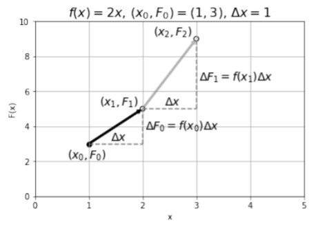
The procedure for determining the anti-derivative \(F(x)\) is illustrated above in Figure A2.3.1. We start by drawing the point that we know the function \(F(x)\) must go through, \((x_0,F_0)\). We then choose a value of \(\Delta x\) and use the derivative, \(f(x)\), to calculate \(\Delta F_0\), the amount by which \(F(x)\) changes when \(x\) changes by \(\Delta x\). Using the derivative \(f(x)\) evaluated at \(x_0\), we have:
\[\begin{aligned} \frac{\Delta F_0}{\Delta x} &\approx f(x_0)\;\;\;\; (\text{in the limit} \Delta x\to 0 )\\[4pt] \therefore \Delta F_0 &= f(x_0) \Delta x\end{aligned}\]
We can then estimate the value of the function \(F_1=F(x_1)\) at the next point, \(x_1=x_0+\Delta x\), as illustrated by the black arrow in Figure A2.3.1
\[\begin{aligned} F_1&=F(x_1)\\[4pt] &=F(x+\Delta x) \\[4pt] &\approx F_0 + \Delta F_0\\[4pt] &\approx F_0+f(x_0)\Delta x\end{aligned}\]
Now that we have determined the value of the function \(F(x)\) at \(x=x_1\), we can repeat the procedure to determine the value of the function \(F(x)\) at the next point, \(x_2=x_1+\Delta x\). Again, we use the derivative evaluated at \(x_1\), \(f(x_1)\), to determine \(\Delta F_1\), and add that to \(F_1\) to get \(F_2=F(x_2)\), as illustrated by the grey arrow in Figure A2.3.1:
\[\begin{aligned} F_2&=F(x_1+\Delta x) \\[4pt] &\approx F_1+\Delta F_1\\[4pt] &\approx F_1+f(x_1)\Delta x\\[4pt] &\approx F_0+f(x_0)\Delta x+f(x_1)\Delta x\end{aligned}\]
Using the summation notation, we can generalize the result and write the function \(F(x)\) evaluated at any point, \(x_N=x_0+N\Delta x\):
\[\begin{aligned} F(x_N) \approx F_0+\sum_{i=1}^{i=N} f(x_{i-1}) \Delta x\end{aligned}\]
The result above will become exactly correct in the limit \(\Delta x\to 0\):
\[F(x_N) = F(x_0)+\lim_{\Delta x\to 0}\sum_{i=1}^{i=N} f(x_{i-1}) \Delta x\]
Let us take a closer look at the sum. Each term in the sum is of the form \(f(x_{i-1})\Delta x\), and is illustrated in Figure A2.3.2 for the same case as in Figure A2.3.1 (that is, Figure A2.3.2 shows \(f(x)\) that we know, and Figure A2.3.1 shows \(F(x)\) that we are trying to find).
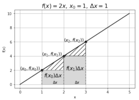
As you can see, each term in the sum corresponds to the area of a rectangle between the function \(f(x)\) and the \(x\) axis (with a piece missing). In the limit where \(\Delta x\to 0\), the missing pieces (shown by the hashed areas in Figure A2.3.2) will vanish and \(f(x_i)\Delta x\) will become exactly the area between \(f(x)\) and the \(x\) axis over a length \(\Delta x\). The sum of the rectangular areas will thus approach the area between \(f(x)\) and the \(x\) axis between \(x_0\) and \(x_N\):
\[\begin{aligned} \lim_{\Delta x\to 0}\sum_{i=1}^{i=N} f(x_{i-1}) \Delta x=\text{Area between f(x) and x axis from $x_0$ to $x_N$}\end{aligned}\]
Re-arranging Equation A2.3.1 gives us a prescription for determining the anti-derivative:
\[\begin{aligned} F(x_N) - F(x_0)&=\lim_{\Delta x\to 0}\sum_{i=1}^{i=N} f(x_{i-1}) \Delta x\end{aligned}\]
We see that if we determine the area between \(f(x)\) and the \(x\) axis from \(x_0\) to \(x_N\), we can obtain the difference between the anti-derivative at two points, \(F(x_N)-F(x_0)\)
The difference between the anti-derivative, \(F(x)\), evaluated at two different values of \(x\) is called the integral of \(f(x)\) and has the following notation:
\[\int_{x_0}^{x_N}f(x) dx=F(x_N) - F(x_0)=\lim_{\Delta x\to 0}\sum_{i=1}^{i=N} f(x_{i-1}) \Delta x\]
As you can see, the integral has labels that specify the range over which we calculate the area between \(f(x)\) and the \(x\) axis. A common notation to express the difference \(F(x_N) - F(x_0)\) is to use brackets:
\[\begin{aligned} \int_{x_0}^{x_N}f(x) dx=F(x_N) - F(x_0) =\big [ F(x) \big]_{x_0}^{x_N}\end{aligned}\]
Recall that we wrote the anti-derivative with the same \(\int\) symbol earlier:
\[\begin{aligned} \int f(x) dx = F(x)\end{aligned}\]
The symbol \(\int f(x) dx\) without the limits is called the indefinite integral. You can also see that when you take the (definite) integral (i.e. the difference between \(F(x)\) evaluated at two points), any constant that is added to \(F(x)\) will cancel. Physical quantities are always based on definite integrals, so when we write the constant \(C\) it is primarily for completeness and to emphasize that we have an indefinite integral.
As an example, let us determine the integral of \(f(x)=2x\) between \(x=1\) and \(x=4\), as well as the indefinite integral of \(f(x)\), which is the case that we illustrated in Figures A2.3.1 and A2.3.2. Using Equation A2.3.2, we have:
\[\begin{aligned} \int_{x_0}^{x_N}f(x) dx&=\lim_{\Delta x\to 0}\sum_{i=1}^{i=N} f(x_{i-1}) \Delta x \\[4pt] &=\lim_{\Delta x\to 0}\sum_{i=1}^{i=N} 2x_{i-1} \Delta x \end{aligned}\]
where we have:
\[\begin{aligned} x_0 &=1 \\[4pt] x_N &=4 \\[4pt] \Delta x &= \frac{x_N-x_0}{N}\end{aligned}\]
Note that \(N\) is the number of times we have \(\Delta x\) in the interval between \(x_0\) and \(x_N\). Thus, taking the limit of \(\Delta x\to 0\) is the same as taking the limit \(N\to\infty\). Let us illustrate the sum for the case where \(N=3\), and thus when \(\Delta x=1\), corresponding to the illustration in Figure A2.3.2:
\[\begin{aligned} \sum_{i=1}^{i=N=3} 2x_{i-1} \Delta x &=2x_0\Delta x+2x_1\Delta x+2x_2\Delta x\\[4pt] &=2\Delta x (x_0+x_1+x_2) \\[4pt] &=2 \frac{x_3-x_0}{N}(x_0+x_1+x_2) \\[4pt] &=2 \frac{(4)-(1)}{(3)}(1+2+3) \\[4pt] &=12\end{aligned}\]
where in the second line, we noticed that we could factor out the \(2\Delta x\) because it appears in each term. Since we only used 4 points, this is a pretty coarse approximation of the integral, and we expect it to be an underestimate (as the missing area represented by the hashed lines in Figure A2.3.2 is quite large).
If we repeat this for a larger value of N, \(N=6\) (\(\Delta x = 0.5\)), we should obtain a more accurate answer:
\[\begin{aligned} \sum_{i=1}^{i=6} 2x_{i-1} \Delta x &=2 \frac{x_6-x_0}{N}(x_0+x_1+x_2+x_3+x_4+x_5)\\[4pt] &=2\frac{4-1}{6} (1+1.5+2+2.5+3+3.5)\\[4pt] &=13.5\end{aligned}\]
Writing this out again for the general case so that we can take the limit \(N\to\infty\), and factoring out the \(2\Delta x\):
\[\begin{aligned} \sum_{i=1}^{i=N} 2x_{i-1} \Delta x &=2 \Delta x\sum_{i=1}^{i=N}x_{i-1}\\[4pt] &=2 \frac{x_N-x_0}{N}\sum_{i=1}^{i=N}x_{i-1}\end{aligned}\]
Now, consider the combination:
\[\begin{aligned} \frac{1}{N}\sum_{i=1}^{i=N}x_{i-1}\end{aligned}\]
that appears above. This corresponds to the arithmetic average of the values from \(x_0\) to \(x_{N-1}\) (sum the values and divide by the number of values). In the limit where \(N\to \infty\), then the value \(x_{N-1}\approx x_N\). The average value of \(x\) in the interval between \(x_0\) and \(x_N\) is simply given by the value of \(x\) at the midpoint of the interval:
\[\begin{aligned} \lim_{N\to\infty}\frac{1}{N}\sum_{i=1}^{i=N}x_{i-1}=\frac{1}{2}(x_N+x_0)\end{aligned}\]
Putting everything together:
\[\begin{aligned} \lim_{N\to\infty}\sum_{i=1}^{i=N} 2x_{i-1} \Delta x &=2 (x_N+x_0)\lim_{N\to\infty}\frac{1}{N}\sum_{i=1}^{i=N}x_{i-1}\\[4pt] &=2 (x_N-x_0)\frac{1}{2}(x_N+x_0)\\[4pt] &=x_N^2 - x_0^2\\[4pt] &=(4)^2 - (1)^2 = 15\end{aligned}\]
where in the last line, we substituted in the values of \(x_0=1\) and \(x_N=4\). Writing this as the integral:
\[\begin{aligned} \int_{x_0}^{x_N}2x dx=F(x_N) - F(x_0)=x_N^2 - x_0^2\end{aligned}\]
we can immediately identify the anti-derivative and the indefinite integral:
\[\begin{aligned} F(x) &= x^2 +C \\[4pt] \int 2xdx&=x^2 +C\end{aligned}\]
This is of course the result that we expected, and we can check our answer by taking the derivative of \(F(x)\):
\[\begin{aligned} \frac{dF}{dx}=\frac{d}{dx}(x^2+C) = 2x\end{aligned}\]
We have thus confirmed that \(F(x)=x^2+C\) is the anti-derivative of \(f(x)=2x\).
The quantity \(\int_{a}^{b}f(t)dt\) is equal to
- the area between the function \(f(t)\) and the \(f\) axis between \(t=a\) and \(t=b\)
- the sum of \(f(t)\Delta t\) in the limit \(\Delta t\to 0\) between \(t=a\) and \(t=b\)
- the difference \(f(b) - f(a)\).
- Answer
-
Common anti-derivative and properties
Table A2.3.1 below gives the anti-derivatives (indefinite integrals) for common functions. In all cases, \(x,\) is the independent variable, and all other variables should be thought of as constants:
| Function, \(f(x)\) | Anti-derivative, \(F(x)\) |
|---|---|
| \(f(x)=a\) | \(F(x)=ax+C\) |
| \(f(x)=x^n\) | \(F(x)=\frac{1}{n+1}x^{n+1}+C\) |
| \(f(x)=\frac{1}{x}\) | \(F(x)=\ln(|x|)+C\) |
| \(f(x)=\sin(x)\) | \(F(x)=-\cos(x)+C\) |
| \(f(x)=\cos(x)\) | \(F(x)=\sin(x)+C\) |
| \(f(x)=\tan(x)\) | \(F(x)=-\ln(|\cos(x)|)+C\) |
| \(f(x)=e^x\) | \(F(x)=e^x+C\) |
| \(f(x)=\ln(x)\) | \(F(x)=x\ln(x)-x+C\) |
Table A2.3.1: Common indefinite integrals of functions.
Note that, in general, it is much more difficult to obtain the anti-derivative of a function than it is to take its derivative. A few common properties to help evaluate indefinite integrals are shown in Table A2.3.2 below.
| Anti-derivative | Equivalent anti-derivative |
|---|---|
| \(\int (f(x)+g(x)) dx\) | \(\int f(x)dx+\int g(x) dx\) (sum) |
| \(\int (f(x)-g(x)) dx\) | \(\int f(x)dx-\int g(x) dx\) (subtraction) |
| \(\int af(x) dx\) | \(a\int f(x)dx\) (multiplication by constant) |
| \(\int f'(x)g(x) dx\) | \(f(x)g(x)-\int f(x)g'(x) dx\) (integration by parts) |
Table A2.3.2: Some properties of indefinite integrals.
Common uses of integrals in Physics - from a sum to an integral
Integrals are extremely useful in physics because they are related to sums. If we assume that our mathematician friends (or computers) can determine anti-derivatives for us, using integrals is not that complicated.
The key idea in physics is that integrals are a tool to easily performing sums. As we saw above, integrals correspond to the area underneath a curve, which is found by summing the (different) areas of an infinite number of infinitely small rectangles. In physics, it is often the case that we need to take the sum of an infinite number of small things that keep varying, just as the areas of the rectangles.
Consider, for example, a rod of length, \(L\), and total mass \(M\), as shown in Figure A2.3.3. If the rod is uniform in density, then if we cut it into, say, two equal pieces, those two pieces will weigh the same. We can define a “linear mass density”, \(\mu\), for the rod, as the mass per unit length of the rod:
\[\begin{aligned} \mu = \frac{M}{L}\end{aligned}\]
The linear mass density has dimensions of mass over length and can be used to find the mass of any length of rod. For example, if the rod has a mass of \(M=5\text{kg}\) and a length of \(L=2\text{m}\), then the mass density is:
\[\begin{aligned} \mu=\frac{M}{L}=\frac{(5\text{kg})}{(2\text{m})}=2.5\text{kg/m}\end{aligned}\]
Knowing the mass density, we can now easily find the mass, \(m\), of a piece of rod that has a length of, say, \(l=10\text{cm}\). Using the mass density, the mass of the \(10\text{cm}\) rod is given by:
\[\begin{aligned} m=\mu l=(2.5\text{kg/m})(0.1\text{m})=0.25\text{kg}\end{aligned}\]
Now suppose that we have a rod of length \(L\) that is not uniform, as in Figure A2.3.3, and that does not have a constant linear mass density. Perhaps the rod gets wider and wider, or it has a holes in it that make it not uniform. Imagine that the mass density of the rod is instead given by a function, \(\mu(x)\), that depends on the position along the rod, where \(x\) is the distance measured from one side of the rod.

Now, we cannot simply determine the mass of the rod by multiplying \(\mu(x)\) and \(L\), since we do not know which value of \(x\) to use. In fact, we have to use all of the values of \(x\), between \(x=0\) and \(x=L\).
The strategy is to divide the rod up into \(N\) pieces of length \(\Delta x\). If we label our pieces of rod with an index \(i\), we can say that the piece that is at position \(x_i\) has a tiny mass, \(\Delta m_i\). We assume that \(\Delta x\) is small enough so that \(\mu(x)\) can be taken as constant over the length of that tiny piece of rod. Then, the tiny piece of rod at \(x=x_i\), has a mass, \(\Delta m_i\), given by:
\[\begin{aligned} \Delta m_i = \mu(x_i) \Delta x\end{aligned}\]
where \(\mu(x_i)\) is evaluated at the position, \(x_i\), of our tiny piece of rod. The total mass, \(M\), of the rod is then the sum of the masses of the tiny rods, in the limit where \(\Delta x\to 0\):
\[\begin{aligned} M &= \lim_{\Delta x\to 0}\sum_{i=1}^{i=N}\Delta m_i \\[4pt] &= \lim_{\Delta x\to 0}\sum_{i=1}^{i=N} \mu(x_i) \Delta x\end{aligned}\]
But this is precisely the definition of the integral (Equation A2.3.1), which we can easily evaluate with an anti-derivative:
\[\begin{aligned} M &=\lim_{\Delta x\to 0}\sum_{i=1}^{i=N} \mu(x_i) \Delta x \\[4pt] &= \int_0^L \mu(x) dx \\[4pt] &= G(L) - G(0)\end{aligned}\]
where \(G(x)\) is the anti-derivative of \(\mu(x)\).
Suppose that the mass density is given by the function:
\[\begin{aligned} \mu(x)=ax^3\end{aligned}\]
with anti-derivative (Table A2.3.1):
\[\begin{aligned} G(x)=a\frac{1}{4}x^4 + C\end{aligned}\]
Let \(a=5\text{kg/m}^{4}\) and let’s say that the length of the rod is \(L=0.5\text{m}\). The total mass of the rod is then:
\[\begin{aligned} M&=\int_0^L \mu(x) dx \\[4pt] &=\int_0^L ax^3 dx \\[4pt] &= G(L)-G(0)\\[4pt] &=\left[ a\frac{1}{4}L^4 \right] - \left[ a\frac{1}{4}0^4 \right]\\[4pt] &=5\text{kg/m}^{4}\frac{1}{4}(0.5\text{m})^4 \\[4pt] &=78\text{g}\\[4pt]\end{aligned}\]
With a little practice, you can solve this type of problem without writing out the sum explicitly. Picture an infinitesimal piece of the rod of length \(dx\) at position \(x\). It will have an infinitesimal mass, \(dm\), given by:
\[\begin{aligned} dm = \mu(x) dx\end{aligned}\]
The total mass of the rod is the then the sum (i.e. the integral) of the mass elements
\[\begin{aligned} M = \int dm\end{aligned}\]
and we really can think of the \(\int\) sign as a sum, when the things being summed are infinitesimally small. In the above equation, we still have not specified the range in \(x\) over which we want to take the sum; that is, we need some sort of index for the mass elements to make this a meaningful definite integral. Since we already know how to express \(dm\) in terms of \(dx\), we can substitute our expression for \(dm\) using one with \(dx\):
\[\begin{aligned} M = \int dm = \int_0^L \mu(x) dx\end{aligned}\]
where we have made the integral definite by specifying the range over which to sum, since we can use \(x\) to “label” the mass elements.
One should note that coming up with the above integral is physics. Solving it is math. We will worry much more about writing out the integral than evaluating its value. Evaluating the integral can always be done by a mathematician friend or a computer, but determining which integral to write down is the physicist’s job!