
18.3: Point Charge
- Page ID
- 14552

\( \newcommand{\vecs}[1]{\overset { \scriptstyle \rightharpoonup} {\mathbf{#1}} } \)
\( \newcommand{\vecd}[1]{\overset{-\!-\!\rightharpoonup}{\vphantom{a}\smash {#1}}} \)
\( \newcommand{\dsum}{\displaystyle\sum\limits} \)
\( \newcommand{\dint}{\displaystyle\int\limits} \)
\( \newcommand{\dlim}{\displaystyle\lim\limits} \)
\( \newcommand{\id}{\mathrm{id}}\) \( \newcommand{\Span}{\mathrm{span}}\)
( \newcommand{\kernel}{\mathrm{null}\,}\) \( \newcommand{\range}{\mathrm{range}\,}\)
\( \newcommand{\RealPart}{\mathrm{Re}}\) \( \newcommand{\ImaginaryPart}{\mathrm{Im}}\)
\( \newcommand{\Argument}{\mathrm{Arg}}\) \( \newcommand{\norm}[1]{\| #1 \|}\)
\( \newcommand{\inner}[2]{\langle #1, #2 \rangle}\)
\( \newcommand{\Span}{\mathrm{span}}\)
\( \newcommand{\id}{\mathrm{id}}\)
\( \newcommand{\Span}{\mathrm{span}}\)
\( \newcommand{\kernel}{\mathrm{null}\,}\)
\( \newcommand{\range}{\mathrm{range}\,}\)
\( \newcommand{\RealPart}{\mathrm{Re}}\)
\( \newcommand{\ImaginaryPart}{\mathrm{Im}}\)
\( \newcommand{\Argument}{\mathrm{Arg}}\)
\( \newcommand{\norm}[1]{\| #1 \|}\)
\( \newcommand{\inner}[2]{\langle #1, #2 \rangle}\)
\( \newcommand{\Span}{\mathrm{span}}\) \( \newcommand{\AA}{\unicode[.8,0]{x212B}}\)
\( \newcommand{\vectorA}[1]{\vec{#1}} % arrow\)
\( \newcommand{\vectorAt}[1]{\vec{\text{#1}}} % arrow\)
\( \newcommand{\vectorB}[1]{\overset { \scriptstyle \rightharpoonup} {\mathbf{#1}} } \)
\( \newcommand{\vectorC}[1]{\textbf{#1}} \)
\( \newcommand{\vectorD}[1]{\overrightarrow{#1}} \)
\( \newcommand{\vectorDt}[1]{\overrightarrow{\text{#1}}} \)
\( \newcommand{\vectE}[1]{\overset{-\!-\!\rightharpoonup}{\vphantom{a}\smash{\mathbf {#1}}}} \)
\( \newcommand{\vecs}[1]{\overset { \scriptstyle \rightharpoonup} {\mathbf{#1}} } \)
\(\newcommand{\longvect}{\overrightarrow}\)
\( \newcommand{\vecd}[1]{\overset{-\!-\!\rightharpoonup}{\vphantom{a}\smash {#1}}} \)
\(\newcommand{\avec}{\mathbf a}\) \(\newcommand{\bvec}{\mathbf b}\) \(\newcommand{\cvec}{\mathbf c}\) \(\newcommand{\dvec}{\mathbf d}\) \(\newcommand{\dtil}{\widetilde{\mathbf d}}\) \(\newcommand{\evec}{\mathbf e}\) \(\newcommand{\fvec}{\mathbf f}\) \(\newcommand{\nvec}{\mathbf n}\) \(\newcommand{\pvec}{\mathbf p}\) \(\newcommand{\qvec}{\mathbf q}\) \(\newcommand{\svec}{\mathbf s}\) \(\newcommand{\tvec}{\mathbf t}\) \(\newcommand{\uvec}{\mathbf u}\) \(\newcommand{\vvec}{\mathbf v}\) \(\newcommand{\wvec}{\mathbf w}\) \(\newcommand{\xvec}{\mathbf x}\) \(\newcommand{\yvec}{\mathbf y}\) \(\newcommand{\zvec}{\mathbf z}\) \(\newcommand{\rvec}{\mathbf r}\) \(\newcommand{\mvec}{\mathbf m}\) \(\newcommand{\zerovec}{\mathbf 0}\) \(\newcommand{\onevec}{\mathbf 1}\) \(\newcommand{\real}{\mathbb R}\) \(\newcommand{\twovec}[2]{\left[\begin{array}{r}#1 \\ #2 \end{array}\right]}\) \(\newcommand{\ctwovec}[2]{\left[\begin{array}{c}#1 \\ #2 \end{array}\right]}\) \(\newcommand{\threevec}[3]{\left[\begin{array}{r}#1 \\ #2 \\ #3 \end{array}\right]}\) \(\newcommand{\cthreevec}[3]{\left[\begin{array}{c}#1 \\ #2 \\ #3 \end{array}\right]}\) \(\newcommand{\fourvec}[4]{\left[\begin{array}{r}#1 \\ #2 \\ #3 \\ #4 \end{array}\right]}\) \(\newcommand{\cfourvec}[4]{\left[\begin{array}{c}#1 \\ #2 \\ #3 \\ #4 \end{array}\right]}\) \(\newcommand{\fivevec}[5]{\left[\begin{array}{r}#1 \\ #2 \\ #3 \\ #4 \\ #5 \\ \end{array}\right]}\) \(\newcommand{\cfivevec}[5]{\left[\begin{array}{c}#1 \\ #2 \\ #3 \\ #4 \\ #5 \\ \end{array}\right]}\) \(\newcommand{\mattwo}[4]{\left[\begin{array}{rr}#1 \amp #2 \\ #3 \amp #4 \\ \end{array}\right]}\) \(\newcommand{\laspan}[1]{\text{Span}\{#1\}}\) \(\newcommand{\bcal}{\cal B}\) \(\newcommand{\ccal}{\cal C}\) \(\newcommand{\scal}{\cal S}\) \(\newcommand{\wcal}{\cal W}\) \(\newcommand{\ecal}{\cal E}\) \(\newcommand{\coords}[2]{\left\{#1\right\}_{#2}}\) \(\newcommand{\gray}[1]{\color{gray}{#1}}\) \(\newcommand{\lgray}[1]{\color{lightgray}{#1}}\) \(\newcommand{\rank}{\operatorname{rank}}\) \(\newcommand{\row}{\text{Row}}\) \(\newcommand{\col}{\text{Col}}\) \(\renewcommand{\row}{\text{Row}}\) \(\newcommand{\nul}{\text{Nul}}\) \(\newcommand{\var}{\text{Var}}\) \(\newcommand{\corr}{\text{corr}}\) \(\newcommand{\len}[1]{\left|#1\right|}\) \(\newcommand{\bbar}{\overline{\bvec}}\) \(\newcommand{\bhat}{\widehat{\bvec}}\) \(\newcommand{\bperp}{\bvec^\perp}\) \(\newcommand{\xhat}{\widehat{\xvec}}\) \(\newcommand{\vhat}{\widehat{\vvec}}\) \(\newcommand{\uhat}{\widehat{\uvec}}\) \(\newcommand{\what}{\widehat{\wvec}}\) \(\newcommand{\Sighat}{\widehat{\Sigma}}\) \(\newcommand{\lt}{<}\) \(\newcommand{\gt}{>}\) \(\newcommand{\amp}{&}\) \(\definecolor{fillinmathshade}{gray}{0.9}\)learning objectives
- Express the electric potential generated by a single point charge in a form of equation
Electric Potential Due to a Point Charge
Overview
Recall that the electric potential is defined as the electric potential energy per unit charge
\[\mathrm { V } = \frac { \mathrm { PE } } { \mathrm { q } }\]
The electric potential tells you how much potential energy a single point charge at a given location will have. The electric potential at a point is equal to the electric potential energy (measured in joules) of any charged particle at that location divided by the charge (measured in coulombs) of the particle. Since the charge of the test particle has been divided out, the electric potential is a “property” related only to the electric field itself and not the test particle. Another way of saying this is that because PE is dependent on q, the q in the above equation will cancel out, so V is not dependent on q.
The potential difference between two points ΔV is often called the voltage and is given by
\[\mathrm{ΔV=V_B−V_A=\dfrac{ΔPE}{q}}\]
Point Charges
Point charges, such as electrons, are among the fundamental building blocks of matter. Furthermore, spherical charge distributions (like on a metal sphere, see figure below) create external electric fields exactly like a point charge. The electric potential due to a point charge is, thus, a case we need to consider. Using calculus to find the work needed to move a test charge q from a large distance away to a distance of r from a point charge Q, and noting the connection between work and potential (W=–qΔV), it can be shown that the electric potential V of a point charge is
\(\mathrm { V } = \frac { \mathrm { k } Q } { \mathrm { r } } \)(point charge)
where k is a constant equal to 9.0×10⁹ N⋅m2/C2 .
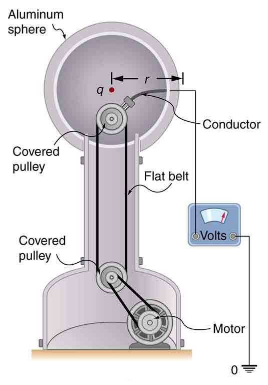
Van de Graaff Generator: The voltage of this demonstration Van de Graaff generator is measured between the charged sphere and ground. Earth’s potential is taken to be zero as a reference. The potential of the charged conducting sphere is the same as that of an equal point charge at its center.
The potential at infinity is chosen to be zero. Thus V for a point charge decreases with distance, whereas E for a point charge decreases with distance squared:
\[\mathrm { E } = \frac { \mathrm { F } } { \mathrm { q } } = \frac { \mathrm { k Q} } { \mathrm { r } ^ { 2 } }\]
The electric potential is a scalar while the electric field is a vector. Note the symmetry between electric potential and gravitational potential – both drop off as a function of distance to the first power, while both the electric and gravitational fields drop off as a function of distance to the second power.
Superposition of Electric Potential
To find the total electric potential due to a system of point charges, one adds the individual voltages as numbers.
learning objectives
- Explain how the total electric potential due to a system of point charges is found
Superposition of Electric Potential
We’ve seen that the electric potential is defined as the amount of potential energy per unit charge a test particle has at a given location in an electric field, i.e.
\[\mathrm { V } = \frac { \mathrm { PE } } { \mathrm { q } }\]
We’ve also seen that the electric potential due to a point charge is
where k is a constant equal to 9.0×10⁹ N⋅m2/C2. The equation for the electric potential of a point charge looks similar to the equation for the electric field generated for a point particle
\[\mathrm{E=\dfrac{F}{q}=\dfrac{kQ}{r^2}}\]
with the difference that the electric field drops off with the square of the distance while the potential drops off linearly with distance. This is analogous to the relationship between the gravitational field and the gravitational potential.
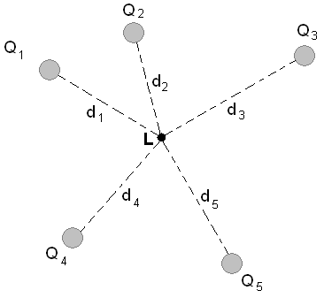
Superposition of Electric Potential: The electric potential at point L is the sum of voltages from each point charge (scalars).
Recall that the electric potential V is a scalar and has no direction, whereas the electric field E is a vector. To find the voltage due to a combination of point charges, you add the individual voltages as numbers. So for example, in the figure above the electric potential at point L is the sum of the potential contributions from charges Q1, Q2, Q3, Q4, and Q5 so that
\[\mathrm { V } _ { \mathrm { L } } = \mathrm { k } \left[ \dfrac { \mathrm{Q}_ { 1 } } { \mathrm { d } _ { 1 } } + \dfrac { \mathrm{Q} _ { 2 } } { \mathrm { d } _ { 2 } } + \dfrac { \mathrm{Q} _ { 3 } } { \mathrm { d } _ { 3 } } + \dfrac { \mathrm{Q} _ { 4 } } { \mathrm { d } _ { 4 } } + \dfrac { \mathrm{Q} _ { 5 } } { \mathrm { d } _ { 5 } } \right]\]
To find the total electric field, you must add the individual fields as vectors, taking magnitude and direction into account. This is consistent with the fact that V is closely associated with energy, a scalar, whereas E is closely associated with force, a vector.
The summing of all voltage contributions to find the total potential field is called the superposition of electric potential. Summing voltages rather than summing the electric simplifies calculations significantly, since addition of potential scalar fields is much easier than addition of the electric vector fields. Note that there are cases where you might need to sum potential contributions from sources other than point charges; however, that is beyond the scope of this section.
Key Points
- Recall that the electric potential is defined as the potential energy per unit charge, i.e. \(\mathrm{V=\frac{PE}{q}}\).
- The potential difference between two points ΔV is often called the voltage and is given b \(\mathrm{ΔV=V_B−V_A=\frac{ΔPE}{q}}\). The potential at an infinite distance is often taken to be zero.
- The case of the electric potential generated by a point charge is important because it is a case that is often encountered. A spherical sphere of charge creates an external field just like a point charge, for example.
- The equation for the electric potential due to a point charge is \(\mathrm{V=\frac{kQ}{r}}\), where k is a constant equal to 9.0×10⁹N⋅m2/C2.
- The electric potential V is a scalar and has no direction, whereas the electric field E is a vector.
- To find the voltage due to a combination of point charges, you add the individual voltages as numbers. So for example, in the electric potential at point L is the sum of the potential contributions from charges Q1, Q2, Q3, Q4, and Q5 so that \(\mathrm { V } _ { \mathrm { L } } = \mathrm { k } \left[ \frac { \mathrm { Q } _ { 1 } } { \mathrm { d } _ { 1 } } + \frac { \mathrm { Q } _ { 2 } } { \mathrm { d } _ { 2 } } + \frac { \mathrm { Q } _ { 3 } } { \mathrm { d } _ { 3 } } + \frac { \mathrm { Q } _ { 4 } } { \mathrm { d } _ { 4 } } + \frac { \mathrm { Q } _ { 5 } } { \mathrm { d } _ { 5 } } \right]\).
- To find the total electric field, you must add the individual fields as vectors, taking magnitude and direction into account. This is consistent with the fact that V is closely associated with energy, a scalar, whereas E is closely associated with force, a vector.
- The summing of all voltage contributions to find the total potential field is called the superposition of electric potential. It is much easier to sum scalars than vectors, so often the preferred method for solving problems with electric fields involves the summing of voltages.
Key Terms
- electric potential: The potential energy per unit charge at a point in a static electric field; voltage.
- voltage: The amount of electrostatic potential between two points in space.
- vector: A directed quantity, one with both magnitude and direction; the between two points.
- scalar: A quantity that has magnitude but not direction; compare vector.
- superposition: The summing of two or more field contributions occupying the same space.
LICENSES AND ATTRIBUTIONS
CC LICENSED CONTENT, SHARED PREVIOUSLY
- Curation and Revision. Provided by: Boundless.com. License: CC BY-SA: Attribution-ShareAlike
CC LICENSED CONTENT, SPECIFIC ATTRIBUTION
- electric potential. Provided by: Wiktionary. Located at: en.wiktionary.org/wiki/electric_potential. License: CC BY-SA: Attribution-ShareAlike
- OpenStax College, College Physics. September 17, 2013. Provided by: OpenStax CNX. Located at: http://cnx.org/content/m42324/latest/?collection=col11406/1.7. License: CC BY: Attribution
- Electric potential. Provided by: Wikipedia. Located at: en.Wikipedia.org/wiki/Electric_potential. License: CC BY-SA: Attribution-ShareAlike
- OpenStax College, College Physics. September 17, 2013. Provided by: OpenStax CNX. Located at: http://cnx.org/content/m42328/latest/?collection=col11406/1.7. License: CC BY: Attribution
- voltage. Provided by: Wiktionary. Located at: en.wiktionary.org/wiki/voltage. License: CC BY-SA: Attribution-ShareAlike
- OpenStax College, College Physics. December 13, 2012. Provided by: OpenStax CNX. Located at: http://cnx.org/content/m42328/latest/?collection=col11406/1.7. License: CC BY: Attribution
- OpenStax College, Electric Potential in a Uniform Electric Field. September 18, 2013. Provided by: OpenStax CNX. Located at: http://cnx.org/content/m42326/latest/. License: CC BY: Attribution
- Electric potential. Provided by: Wikipedia. Located at: en.Wikipedia.org/wiki/Electric_potential. License: CC BY-SA: Attribution-ShareAlike
- OpenStax College, College Physics. September 18, 2013. Provided by: OpenStax CNX. Located at: http://cnx.org/content/m42324/latest/?collection=col11406/1.7. License: CC BY: Attribution
- scalar. Provided by: Wiktionary. Located at: en.wiktionary.org/wiki/scalar. License: CC BY-SA: Attribution-ShareAlike
- Boundless. Provided by: Boundless Learning. Located at: www.boundless.com//physics/definition/superposition. License: CC BY-SA: Attribution-ShareAlike
- vector. Provided by: Wiktionary. Located at: en.wiktionary.org/wiki/vector. License: CC BY-SA: Attribution-ShareAlike
- OpenStax College, College Physics. December 13, 2012. Provided by: OpenStax CNX. Located at: http://cnx.org/content/m42328/latest/?collection=col11406/1.7. License: CC BY: Attribution
- Potencial eletrico resultante. Provided by: Wikimedia. Located at: commons.wikimedia.org/wiki/File:Potencial_eletrico_resultante.PNG. License: Public Domain: No Known Copyright