3.5: Energy Landscapes

In the previous section we proved that the total energy is conserved. In the section before that, we looked at potential energies. Typically, the potential energy is a function of your position in space. When we plot it as a function of spatial coordinates, we get an energy landscape, measuring an amount of energy on the vertical axis. Of course we can also plot the total energy of the system - and since that is conserved, it is the same everywhere, and thus becomes a horizontal line or plane. Because kinetic energy cannot be negative, any point where the potential energy is higher than the total energy is not allowed: the system cannot reach this point. When the potential energy equals the total energy, the kinetic energy (and thus the speed) has to be zero. Whenever the potential energy is lower than the total energy, there is a positive kinetic energy and thus a positive speed.

Figure $\PageIndex{1}$: An example of a potential energy landscape. In this figure, the total energy would be represented by a horizontal line; the kinetic energy by the distance between the potential and total energy. Equilibrium points (dots) occur at extrema of the potential energy,when its derivative (the force) is zero. The green dots indicate unstable equilibrium points (maxima, where the second derivative is negative), the orange points metastable equilibria (local minima) and the red point the single globally stable equilibrium of this system.

Probably the simplest energy landscape is that of the harmonic oscillator (mass on a spring) - it’s a simple parabola. The point at which the horizontal line representing the total energy crosses the parabola corresponds to the extrema of the oscillation: these are its turning points. The bottom of the parabola is its mid-point, and you can immediately see that that’s where the kinetic energy (and thus the speed) will be highest.

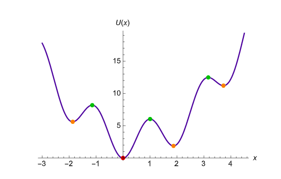
Of course you can have more complex energy landscapes than that. In particular, you can have a landscape with multiple extrema, see for example Figure $\PageIndex{1}$ A particle that is being acted upon by forces described by this potential energy, follows a trajectory in this landscape, which can be visualized as a ball rolling over the hills and valleys of the landscape. Think back to the harmonic oscillator example. If we let go of a ball in a parabolic vase at some point on the slope, the ball will roll down and pick up speed, then roll up the opposite slope and lose speed, until it reaches the same height where its speed will again be zero. The same is true in more complicated landscapes. Particularly interesting are local maxima. If you put a ball exactly on top of one of them, it will stay there - it is a fixed point, but an unstable one, as any arbitrarily small perturbation will push it down. If you let go of a ball at a level above a local maximum, it may hop over it to the next minimum,but if your initial position (your initial energy) was too low, your ball can get stuck oscillating about a local minimum - a metastable point.

Energy landscapes are even useful when the total energy is not conserved - for example because of friction terms. Friction causes energy to dissipate from the system, which is equivalent to having your ball move in the landscape with friction. For low friction, your ball will oscillate, but get less high every time, until it comes to rest at the minimum. For high friction, it won’t even oscillate, but just get to the minimum - exactly what an over damped system in real life does.

Example $\PageIndex{1}$: Worked example: the Lennard-Jones Potential

The Lennard-Jones potential energy is a commonly used model to describe the interactions between uncharged atoms and molecules. This potential energy can be written in two equivalent ways:

$$U_{\mathrm{LJ}}(r)=\frac{A}{r^{12}}-\frac{B}{r^{6}}=4 \varepsilon\left[\left(\frac{\sigma}{r}\right)^{12}-\left(\frac{\sigma}{r}\right)^{6}\right] \nonumber$$

where $r$ is the distance between the atoms or molecules, and A, B, $\varepsilon$, and $\sigma$ are positive constants.

1. Find the dimensions of A, B, $\varepsilon$, and $\sigma$.
2. Express $\varepsilon$ and $\sigma$ in A and B.
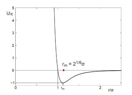
3. Sketch the potential (in its second form) as a function of $\frac{r}{\sigma}$, and use this sketch to give a physical interpretation of $\varepsilon$ and $\sigma$.
4. Does the Lennard-Jones potential lead to attractive or repulsive forces at short distances? And what about long distances?
5. Find all equilibrium points of this potential energy, and determine their stability.

Solution

Figure $\PageIndex{2}$: Sketch of the Lennard-Jones potential energy.

1. $$\begin{array}{l}{[U]=\text { Energy } \Longrightarrow[U]=M \times \frac{L}{T^{2}} \times L=\frac{M L^{2}}{T^{2}}} \\ {[A]=\text { Energy } \times \text { Length }^{12} \Longrightarrow[A]=\frac{M L^{2}}{T^{2}}} \\ {[B]=\text { Energy } \times \text { Length }^{6} \Longrightarrow[A]=\frac{M L^{8}}{T^{2}}}\end{array}\nonumber$$ Because the powers of the terms $\left(\left(\frac{\sigma}{r}\right)^{12}\right) \text { and }\left(\left(\frac{\sigma}{r}\right)^{6}\right)$ are different, while we add them together, they haveto be dimensionless, so $$[\sigma]=L \text { and }[\varepsilon]=[U]=\frac{M L^{2}}{T^{2}}\nonumber$$ .
2. $$\begin{array}{l}{4 \epsilon \sigma^{12}=A \text { and } 4 \varepsilon \sigma^{6}=B} \\ {\frac{A}{B}=\sigma^{6} \Longrightarrow \sigma=\left(\frac{A}{B}\right)^{1 / 6}}\end{array}\nonumber$$ By substituting $\sigma$ in the expressions for either A or B we can derive an expression for $\varepsilon$: $$\begin{array}{l}{4 \sigma^{6} \varepsilon=B} \\ {4 \varepsilon A=B^{2} \Longrightarrow \varepsilon=\frac{B^{2}}{4 A}}\end{array}\nonumber$$
3. (c) Figure $\PageIndex{2}$. Interpretation:≤is a measure for the depth of the potential well.æsets the length scale andtherefore the position of the equilibrium point.
4. Method 1: We calculate the force as minus the derivative of the potential energy: $$F=-\frac{\partial U}{\partial r}=4 \varepsilon\left(\frac{12 \sigma^{12}}{r^{13}}-\frac{6 \sigma^{6}}{r^{7}}\right)\nonumber$$ For small r we have $r^{-13} \gt \gt r^{-7}$, so F is positive and therefore repulsive. Conversely, for larger we have $r^{-13} \lt \lt r^{-7}$, so F is negative and therefore attractive. Method 2: Use the sketch in (c) to to see that the slope of the potential is negative for small r, which implies a repulsive force, and the slope of the potential is positive for larger, which implies an attractive force.
5. For an equilibrium point we have $$0=\frac{\partial U}{\partial r}=4 \varepsilon\left(\frac{12 \sigma^{12}}{r^{13}}-\frac{6 \sigma^{6}}{r^{7}}\right)=24 \frac{\varepsilon \sigma^{6}}{r^{7}}\left(\frac{2 \sigma^{6}}{r^{6}}-1\right)\nonumber$$ so there is only one equilibrium point, at $$r_{\mathrm{eq}}=2^{1 / 6} \sigma\nonumber$$ To determine the stability at this point, we consider the second derivative of U(r): $$\left.\frac{\partial^{2} U}{\partial r^{2}}\right|_{r=r_{\mathrm{eq}}}=4 \varepsilon\left.\left(42 \frac{\sigma^{6}}{r^{8}}-156 \frac{\sigma^{12}}{r^{14}}\right)\right|_{r=r_{\mathrm{eq}}}=4 \varepsilon\left(\frac{42}{2^{4 / 3} \sigma^{2}}-\frac{156}{2^{7 / 3} \sigma^{2}}\right)=-36 \cdot 2^{2 / 3} \frac{\varepsilon}{\sigma^{2}}<0\nonumber$$ which means that the equilibrium point is stable. Alternatively, we could have determined the stability by considering the graph drawn at (c), from which we can see that the equilibrium point corresponds toa global minimum of the potential energy and hence is stable.