11.2: Flow in Tubes
- Page ID
- 14502
\( \newcommand{\vecs}[1]{\overset { \scriptstyle \rightharpoonup} {\mathbf{#1}} } \)
\( \newcommand{\vecd}[1]{\overset{-\!-\!\rightharpoonup}{\vphantom{a}\smash {#1}}} \)
\( \newcommand{\id}{\mathrm{id}}\) \( \newcommand{\Span}{\mathrm{span}}\)
( \newcommand{\kernel}{\mathrm{null}\,}\) \( \newcommand{\range}{\mathrm{range}\,}\)
\( \newcommand{\RealPart}{\mathrm{Re}}\) \( \newcommand{\ImaginaryPart}{\mathrm{Im}}\)
\( \newcommand{\Argument}{\mathrm{Arg}}\) \( \newcommand{\norm}[1]{\| #1 \|}\)
\( \newcommand{\inner}[2]{\langle #1, #2 \rangle}\)
\( \newcommand{\Span}{\mathrm{span}}\)
\( \newcommand{\id}{\mathrm{id}}\)
\( \newcommand{\Span}{\mathrm{span}}\)
\( \newcommand{\kernel}{\mathrm{null}\,}\)
\( \newcommand{\range}{\mathrm{range}\,}\)
\( \newcommand{\RealPart}{\mathrm{Re}}\)
\( \newcommand{\ImaginaryPart}{\mathrm{Im}}\)
\( \newcommand{\Argument}{\mathrm{Arg}}\)
\( \newcommand{\norm}[1]{\| #1 \|}\)
\( \newcommand{\inner}[2]{\langle #1, #2 \rangle}\)
\( \newcommand{\Span}{\mathrm{span}}\) \( \newcommand{\AA}{\unicode[.8,0]{x212B}}\)
\( \newcommand{\vectorA}[1]{\vec{#1}} % arrow\)
\( \newcommand{\vectorAt}[1]{\vec{\text{#1}}} % arrow\)
\( \newcommand{\vectorB}[1]{\overset { \scriptstyle \rightharpoonup} {\mathbf{#1}} } \)
\( \newcommand{\vectorC}[1]{\textbf{#1}} \)
\( \newcommand{\vectorD}[1]{\overrightarrow{#1}} \)
\( \newcommand{\vectorDt}[1]{\overrightarrow{\text{#1}}} \)
\( \newcommand{\vectE}[1]{\overset{-\!-\!\rightharpoonup}{\vphantom{a}\smash{\mathbf {#1}}}} \)
\( \newcommand{\vecs}[1]{\overset { \scriptstyle \rightharpoonup} {\mathbf{#1}} } \)
\( \newcommand{\vecd}[1]{\overset{-\!-\!\rightharpoonup}{\vphantom{a}\smash {#1}}} \)
\(\newcommand{\avec}{\mathbf a}\) \(\newcommand{\bvec}{\mathbf b}\) \(\newcommand{\cvec}{\mathbf c}\) \(\newcommand{\dvec}{\mathbf d}\) \(\newcommand{\dtil}{\widetilde{\mathbf d}}\) \(\newcommand{\evec}{\mathbf e}\) \(\newcommand{\fvec}{\mathbf f}\) \(\newcommand{\nvec}{\mathbf n}\) \(\newcommand{\pvec}{\mathbf p}\) \(\newcommand{\qvec}{\mathbf q}\) \(\newcommand{\svec}{\mathbf s}\) \(\newcommand{\tvec}{\mathbf t}\) \(\newcommand{\uvec}{\mathbf u}\) \(\newcommand{\vvec}{\mathbf v}\) \(\newcommand{\wvec}{\mathbf w}\) \(\newcommand{\xvec}{\mathbf x}\) \(\newcommand{\yvec}{\mathbf y}\) \(\newcommand{\zvec}{\mathbf z}\) \(\newcommand{\rvec}{\mathbf r}\) \(\newcommand{\mvec}{\mathbf m}\) \(\newcommand{\zerovec}{\mathbf 0}\) \(\newcommand{\onevec}{\mathbf 1}\) \(\newcommand{\real}{\mathbb R}\) \(\newcommand{\twovec}[2]{\left[\begin{array}{r}#1 \\ #2 \end{array}\right]}\) \(\newcommand{\ctwovec}[2]{\left[\begin{array}{c}#1 \\ #2 \end{array}\right]}\) \(\newcommand{\threevec}[3]{\left[\begin{array}{r}#1 \\ #2 \\ #3 \end{array}\right]}\) \(\newcommand{\cthreevec}[3]{\left[\begin{array}{c}#1 \\ #2 \\ #3 \end{array}\right]}\) \(\newcommand{\fourvec}[4]{\left[\begin{array}{r}#1 \\ #2 \\ #3 \\ #4 \end{array}\right]}\) \(\newcommand{\cfourvec}[4]{\left[\begin{array}{c}#1 \\ #2 \\ #3 \\ #4 \end{array}\right]}\) \(\newcommand{\fivevec}[5]{\left[\begin{array}{r}#1 \\ #2 \\ #3 \\ #4 \\ #5 \\ \end{array}\right]}\) \(\newcommand{\cfivevec}[5]{\left[\begin{array}{c}#1 \\ #2 \\ #3 \\ #4 \\ #5 \\ \end{array}\right]}\) \(\newcommand{\mattwo}[4]{\left[\begin{array}{rr}#1 \amp #2 \\ #3 \amp #4 \\ \end{array}\right]}\) \(\newcommand{\laspan}[1]{\text{Span}\{#1\}}\) \(\newcommand{\bcal}{\cal B}\) \(\newcommand{\ccal}{\cal C}\) \(\newcommand{\scal}{\cal S}\) \(\newcommand{\wcal}{\cal W}\) \(\newcommand{\ecal}{\cal E}\) \(\newcommand{\coords}[2]{\left\{#1\right\}_{#2}}\) \(\newcommand{\gray}[1]{\color{gray}{#1}}\) \(\newcommand{\lgray}[1]{\color{lightgray}{#1}}\) \(\newcommand{\rank}{\operatorname{rank}}\) \(\newcommand{\row}{\text{Row}}\) \(\newcommand{\col}{\text{Col}}\) \(\renewcommand{\row}{\text{Row}}\) \(\newcommand{\nul}{\text{Nul}}\) \(\newcommand{\var}{\text{Var}}\) \(\newcommand{\corr}{\text{corr}}\) \(\newcommand{\len}[1]{\left|#1\right|}\) \(\newcommand{\bbar}{\overline{\bvec}}\) \(\newcommand{\bhat}{\widehat{\bvec}}\) \(\newcommand{\bperp}{\bvec^\perp}\) \(\newcommand{\xhat}{\widehat{\xvec}}\) \(\newcommand{\vhat}{\widehat{\vvec}}\) \(\newcommand{\uhat}{\widehat{\uvec}}\) \(\newcommand{\what}{\widehat{\wvec}}\) \(\newcommand{\Sighat}{\widehat{\Sigma}}\) \(\newcommand{\lt}{<}\) \(\newcommand{\gt}{>}\) \(\newcommand{\amp}{&}\) \(\definecolor{fillinmathshade}{gray}{0.9}\)learning objectives
- Contrast turbulent and laminar flow in constant velocity
Virtually all moving fluids exhibit viscosity, which is a measure of the resistance of a fluid to flow. Viscosity is a basic property necessary for the analysis of fluid flow.
Measure of Fluid Friction
It describes a fluid’s internal resistance to movement and can be thought of as a measure of fluid friction. The greater the viscosity, the ‘thicker’ the fluid and the more the fluid will resist movement.
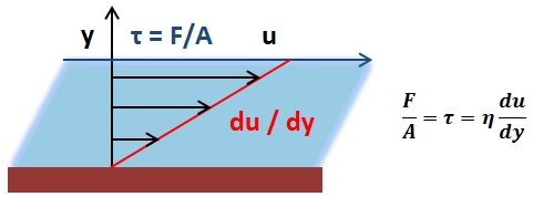
Mathematically, viscosity is a proportionality constant relating an applied shear stress to the resulting shear velocity and is given, along with a representative diagram, (see ). As shown, when a force is applied to a fluid, creating a shear stress, the fluid will undergo a certain displacement. The viscosity of the fluid is then its inherent resistance to undergo this displacement.

Representation of Viscosity: A proportionality constant relating an applied shear stress to the resulting shear velocity.
Different fluids exhibit different viscous behavior yet, in this analysis, only Newtonian fluids (fluids with constant velocity independent of applied shear stress) will be considered. Viscosity in fluids generally decreases with increasing temperature. The study of the viscous nature of fluids is called rheology.
In analyzing the properties of moving fluids, it is necessary to determine the nature of flow of the fluid. This is generally split into two categories, laminar and turbulent flow.
Turbulent Flow
Turbulent flow is characterized by irregular flow of a fluid in which there are both inconsistent flow patterns and velocity variations throughout the volume of the fluid in motion. Analysis of turbulent flow can be very complex and often requires advanced mathematical analysis to simulate flow in systems on a near case-by-case basis.
It occurs when the Reynolds number is above a certain critical threshold while mixed turbulent–laminar flow occurs within a range of Reynolds number below this threshold value. At the lower limit of this mixed turbulent–laminar flow Reynolds number region there is another critical threshold value, below which only laminar flow is possible.
Laminar Flow
Laminar flow consists of a regular-flow pattern with constant-flow velocity throughout the fluid volume and is much easier to analyze than turbulent flow.

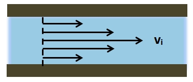
Relative Magnitudes of Velocity Vectors: Laminar fluid flow in a circular pipe at the same direction.
Laminar flow is often encountered in common hydraulic systems, such as where fluid flow is through an enclosed, rigid pipe; the fluid is incompressible, has constant viscosity, and the Reynolds number is below this lower critical threshold value. It is characterized by the flow of a fluid in parallel layers, in which there is no disruption or interaction between the different layers, and in which each layer flows at a different velocity along the same direction. The variation in velocity between adjacent parallel layers is due to the viscosity of the fluid and resulting shear forces.
This figure (see ) gives a representation of the relative magnitudes of the velocity vectors of each of these layers for laminar fluid flow through a circular pipe, in a direction parallel to the pipe axis.

Poiseuille’s Equation: Can be used to determine the pressure drop of a constant viscosity fluid exhibiting laminar flow through a rigid pipe.
Considering laminar flow of a constant density, incompressible fluid such as for a Newtonian fluid traveling in a pipe, with a Reynolds number below the upper limit level for fully laminar flow, the pressure difference between two points along the pipe can be found from the volumetric flow rate, or vice versa. For such a system with a pipe radius of r, fluid viscosity η, distance between the two points along the pipe Δx = x2 – x1, and the volumetric flow rate Q, of the fluid, the pressure difference between the two points along the pipe Δp is given by Poiseuille’s equation (see ).
This equation is valid for laminar flow of incompressible fluids only, and may be used to determine a number of properties in the hydraulic system, if the others are known or can be measured. In practice, Poiseuille’s equation holds for most systems involving laminar flow of a fluid, except at regions where features disrupting laminar flow, such as at the ends of a pipe, are present.
Poiseuille’s equation as given in this example (see ) is analogous to Ohm ‘s equation for determining the resistance in an electronic circuit and is of great practical use in hydraulic-circuit analysis.

Poiseuille’s Equation: Analogous to Ohm’s Law Analogy
Blood Flow
Blood flow is the continuous running of blood through the cardiovascular system, which consists of the vessels and the heart.
learning objectives
- Outline how normal plasma behaves in a mammalian cardiovascular system
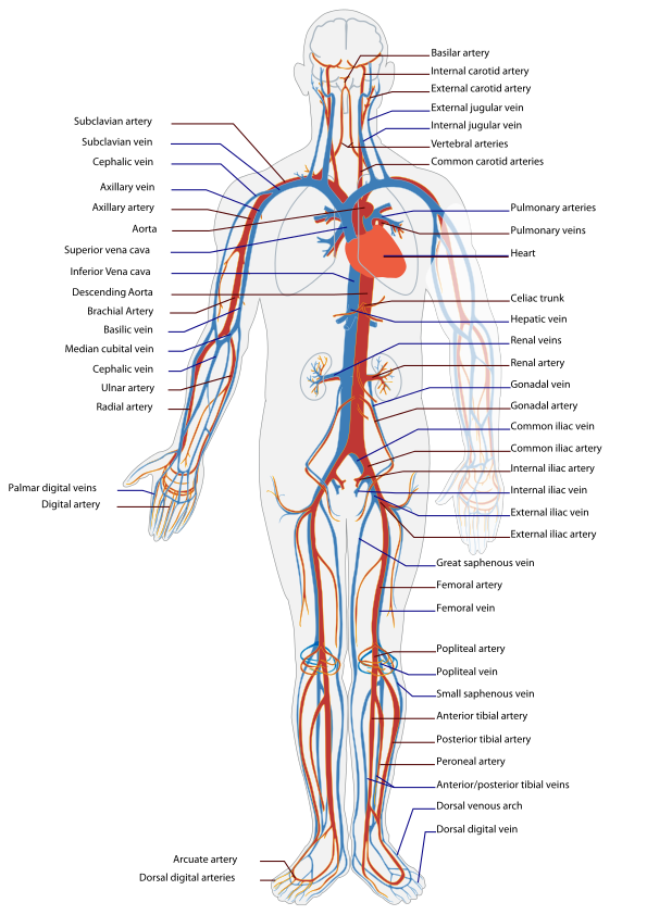
Blood flow is the continuous running of blood through vessels in the cardiovascular system (the mammalian cardiovascular system is shown in ). Blood is the viscous fluid composed of plasma and cells. The composition of the blood includes plasma, red blood cells, white blood cells and platelets. In microcirculation, the properties of the blood cells have an important influence on flow.

An illustrative overview of the mammalian cardiovascular system: Keep in mind that both circular paths are working simultaneously and not in a sequential manner as the numbering in the illustration might suggest. Both the ventricles are working together in harmony; as tiny amounts of blood are moving in the pulmonary circuit, the remainder of the blood moves through the systemic circuit.
The cardiovascular system, which consists of blood vessels and the heart, helps to distribute nutrients, O2, and other products of metabolism. The blood moves in the blood vessels, while the heart serves as the pump for the blood. The vessel walls of the heart are elastic and movable, therefore causing the blood and the wall to exert forces on each other and in turn influencing their respective motion.
The major quantity of interest in describing the motion of blood particles is velocity—the rate of change of the position of an object with time:
\[\mathrm{v=\dfrac{Δx}{Δt}}\]
Blood velocities in arteries are higher during systole than during diastole. One parameter to quantify this difference is pulsatility index (PI), which is equal to the difference between the peak systolic velocity and the minimum diastolic velocity divided by the mean velocity during the cardiac cycle.
Another important parameter is the acceleration—the rate of change of velocity: \(\mathrm{a=\frac{Δv}{Δt}}\)
Normal plasma behaves like a Newtonian fluid at rates of shear. Typical values for the viscosity of normal human plasma at 37°C is 1.2Nsm-2. The viscosity of normal plasma varies with temperature in the same way as does that of its solvent, water. (a 5°C increase of temperature in the physiological range reduces plasma viscosity by about 10%).
The osmotic pressure of the plasma affects the mechanics of the circulation in several ways. An alteration of the osmotic pressure difference across the membrane of a blood cell causes a shift of water and a change in cell volume. The change, both in shape and flexibility, affects the mechanical properties of whole blood. Therefore, a change in plasma osmotic pressure alters the hematocrit (the volume concentration of red cells in the whole blood) by redistributing water between the intravascular and extravascular spaces. This in turn affects the mechanics of the whole blood.
Key Points
- Viscosity is the resistance of a fluid to flow. Virtually all fluids have viscosity which generally changes as a function of temperature; although different types of fluids exhibit different types of fluid–shear velocity dependencies.
- Laminar flow of a fluid is characterized by its flow in parallel layers in which there is no disruption or interaction between the different layers, and in which each layer flows at a different velocity along the same direction.
- Poiseuille’s equation pertains to moving incompressible fluids exhibiting laminar flow. It relates the difference in pressure at different spatial points to volumetric flow rate for fluids in motion in certain cases, such as in the flow of fluid through a rigid pipe.
- The major quantity of interest in describing the motion of blood particles is the velocity – the rate of change of the position of an object with time: \(\mathrm{v=\frac{Δx}{Δt}}\).
- Blood velocities in arteries are higher during systole than during diastole.
- The mechanics of the circulation depends on osmotic pressure of plasma.
Key Terms
- viscosity: The property of a fluid that resists the force which tends to cause it to flow.
- shear stress: The external force acting on an object or surface parallel to the slope or plane in which it lies; the stress tending to produce shear.
- Reynolds Number: A dimensionless number, \(\mathrm{\frac{vρl}{η}}\), where v is the fluid velocity, ρ the density, η the viscosity and l a dimension of the system. The value of the number indicates the type of fluid flow.
- systole: The rhythmic contraction of the heart, by which blood is driven through the arteries.
- vessel: A tube or canal that carries fluid in an animal or plant.
- diastole: The phase or process of relaxation and dilation of the heart chambers, between contractions, during which they fill with blood; an instance of the process.
LICENSES AND ATTRIBUTIONS
CC LICENSED CONTENT, SHARED PREVIOUSLY
- Curation and Revision. Provided by: Boundless.com. License: CC BY-SA: Attribution-ShareAlike
CC LICENSED CONTENT, SPECIFIC ATTRIBUTION
- Poiseuille. Provided by: Wikipedia. Located at: en.Wikipedia.org/wiki/Poiseuille. License: CC BY-SA: Attribution-ShareAlike
- Laminar flow. Provided by: Wikipedia. Located at: en.Wikipedia.org/wiki/Laminar_flow. License: CC BY-SA: Attribution-ShareAlike
- Viscosity. Provided by: Wikipedia. Located at: en.Wikipedia.org/wiki/Viscosity. License: CC BY-SA: Attribution-ShareAlike
- Poiseuille. Provided by: Wikipedia. Located at: en.Wikipedia.org/wiki/Poiseuille. License: CC BY-SA: Attribution-ShareAlike
- viscosity. Provided by: Wiktionary. Located at: en.wiktionary.org/wiki/viscosity. License: CC BY-SA: Attribution-ShareAlike
- Boundless. Provided by: Boundless Learning. Located at: www.boundless.com//physics/definition/reynolds-number. License: CC BY-SA: Attribution-ShareAlike
- shear stress. Provided by: Wiktionary. Located at: en.wiktionary.org/wiki/shear_stress. License: CC BY-SA: Attribution-ShareAlike
- Provided by: N/A. Located at: N/A. License: CC BY-SA: Attribution-ShareAlike
- Provided by: N/A. Located at: N/A. License: CC BY-SA: Attribution-ShareAlike
- Provided by: N/A. Located at: N/A. License: CC BY-SA: Attribution-ShareAlike
- Provided by: N/A. Located at: N/A. License: CC BY-SA: Attribution-ShareAlike
- Blood flow. Provided by: Wikipedia. Located at: en.Wikipedia.org/wiki/Blood_flow. License: CC BY-SA: Attribution-ShareAlike
- diastole. Provided by: Wiktionary. Located at: en.wiktionary.org/wiki/diastole. License: CC BY-SA: Attribution-ShareAlike
- systole. Provided by: Wiktionary. Located at: en.wiktionary.org/wiki/systole. License: CC BY-SA: Attribution-ShareAlike
- vessel. Provided by: Wiktionary. Located at: en.wiktionary.org/wiki/vessel. License: CC BY-SA: Attribution-ShareAlike
- Provided by: N/A. Located at: N/A. License: CC BY-SA: Attribution-ShareAlike
- Provided by: N/A. Located at: N/A. License: CC BY-SA: Attribution-ShareAlike
- Provided by: N/A. Located at: N/A. License: CC BY-SA: Attribution-ShareAlike
- Provided by: N/A. Located at: N/A. License: CC BY-SA: Attribution-ShareAlike
- Circulatory System en. Provided by: Wikimedia. Located at: commons.wikimedia.org/wiki/File:Circulatory_System_en.svg. License: Public Domain: No Known Copyright


