13.3: Gravitational Flux

Last updated
Save as PDF

Page ID: 32822

\( \newcommand{\vecs}[1]{\overset { \scriptstyle \rightharpoonup} {\mathbf{#1}} } \) \( \newcommand{\vecd}[1]{\overset{-\!-\!\rightharpoonup}{\vphantom{a}\smash {#1}}} \)\(\newcommand{\id}{\mathrm{id}}\) \( \newcommand{\Span}{\mathrm{span}}\) \( \newcommand{\kernel}{\mathrm{null}\,}\) \( \newcommand{\range}{\mathrm{range}\,}\) \( \newcommand{\RealPart}{\mathrm{Re}}\) \( \newcommand{\ImaginaryPart}{\mathrm{Im}}\) \( \newcommand{\Argument}{\mathrm{Arg}}\) \( \newcommand{\norm}[1]{\| #1 \|}\) \( \newcommand{\inner}[2]{\langle #1, #2 \rangle}\) \( \newcommand{\Span}{\mathrm{span}}\) \(\newcommand{\id}{\mathrm{id}}\) \( \newcommand{\Span}{\mathrm{span}}\) \( \newcommand{\kernel}{\mathrm{null}\,}\) \( \newcommand{\range}{\mathrm{range}\,}\) \( \newcommand{\RealPart}{\mathrm{Re}}\) \( \newcommand{\ImaginaryPart}{\mathrm{Im}}\) \( \newcommand{\Argument}{\mathrm{Arg}}\) \( \newcommand{\norm}[1]{\| #1 \|}\) \( \newcommand{\inner}[2]{\langle #1, #2 \rangle}\) \( \newcommand{\Span}{\mathrm{span}}\)\(\newcommand{\AA}{\unicode[.8,0]{x212B}}\)

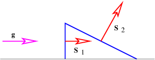
The next concept we need to discuss is the gravitational flux. Figure 13.2 shows a rectangular area \(S \) with a vector \(S\) perpendicular to the rectangle. The vector \(S\) is defined to have length \(S\), so it is a compact way of representing the size and orientation of a rectangle in three dimensional space. The vector \(S\) could point either upward or downward, and the choice of directions turns out to be important. This is why we say that \(S\) represents a directed area.

Figure 13.2: Definition sketch for the gravitational flux through the directed area \(S\).

Figure 13.2 also shows a vector \(g\), representing the gravitational field on the surface of the rectangle. Its value is assumed here not to vary with position on the rectangle. The angle \(θ \) is the angle between the vectors \(S\) and \(g\).

Figure 13.3: Two areas with the same projected area normal to \(g\). Is the flux through area 2 greater than, less than, or equal to the flux through area 1? (The two areas are being viewed edge-on and are assumed to have some dimension \(d \) in the direction normal to the page.)

The gravitational flux through the rectangle is defined as

\[Φg = S ⋅ g = Sg cosθ = Sgn, \label{13.3}\]

where \(g\) _n = \(g\) cos \(θ \) is the component of \(g\) normal to the rectangle. The flux is thus larger for larger areas and for larger gravitational fields. However, only the component of the gravitational field normal to the rectangle (i. e., parallel to \(S\) ) counts in this calculation. A consequence is that the gravitational flux through area 1, \(S\) ₁ ⋅ \(g\), in figure 13.3 is the same as the flux through area 2, \(S\) ₂ ⋅ \(g\).

The significance of the directedness of the area is now clear. If the vector \(S\) pointed in the opposite direction, the flux would have the opposite sign. When defining the flux through a rectangle, it is necessary to define which way the flux is going. This is what the direction of \(S\) does — a positive flux is defined as going from the side opposite \(S\) to the side of \(S\).

An analogy with flowing water may be helpful. Imagine a rectangular channel of cross-sectional area \(S \) through which water is flowing at velocity \(v\). The flux of water through the channel, which is defined as the volume of water per unit time passing through the cross-sectional area, is Φ_w = \(vS\). The water velocity takes the place of the gravitational field in this case, and its direction is here assumed to be normal to the rectangular cross-section of the channel. The field thus expresses an intensity (e. g., the velocity of the water or the strength of the gravitational field), while the flux expresses an amount (the volume of water per unit time in the fluid dynamical case). The gravitational flux is thus the amount of some gravitational influence , while the gravitational field is its strength. We now try to more clearly understand to what this amount really refers.

We need to briefly consider the case in which the gravitational field varies from one point to another on the rectangular surface. In this case a proper calculation of the flux through the surface cannot be made using equation 13.3} directly. Instead, we must break the surface into a grid of sub-surfaces. If the grid is sufficiently fine, the gravitational field will be nearly constant over each sub-surface and equation 13.3} can be applied separately to each of these. The total flux is then the sum of all the individual fluxes.

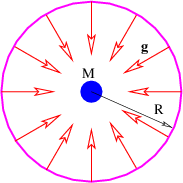
Figure 13.4: Calculation of the gravitational flux through the surface of a sphere with a mass at the center.

There is actually no need for the area in figure 13.2 to be rectangular. We can calculate the gravitational flux through the surface of a sphere of radius \(R \) with a mass \(M \) at the center. As illustrated in figure 13.4, the gravitational field points inward toward the mass. It has magnitude \(g \) = \(GM∕R\) ², so if we desire to calculate the gravitational flux out of the sphere, we must introduce a minus sign. Finally, the area of a sphere of radius \(R \) is \(S \) = 4\(πR\) ², so the flux is

\[Φg = - gS = - (GM ∕R2 )(4πR2 ) = - 4 πGM. \label{13.4}\]

Notice that this flux doesn’t depend on how big the sphere is — the factor of \(R\) ² in the area cancels with the factor of 1\(∕R\) ² in the gravitational field. This is a hint that something profound is going on. The size of the surface enclosing the mass is unimportant, and neither is its shape — the answer is always the same — the gravitational flux outward through any closed surface surrounding a mass \(M \) is just Φ_g = -4\(πGM\) ! This is an example of Gauss’s law applied to gravity.

Figure 13.5: Three cases of a mass \(M \) and a closed surface. In the left and center examples the mass is inside the closed surface and the outward flux through the surface is Φ_g = -4\(πGM\). In the right example the mass is outside the surface and the outward flux through the surface is zero.

It is possible to formally prove this result using arguments like those posed in figure 13.3, but perhaps the easiest way to understand this result is via the analogy with the flow of water. If we think of the mass as something which destroys water at a certain rate, then there must be an inward flow of water through the surfaces in the left and center examples in figure 13.5. Furthermore, the volume of water per unit time flowing inward through these surfaces is the same in the two examples, because the rate at which water is being destroyed is the same. In the right case the mass is not contained inside the surface and though water flows into the volume bounded by the surface, it also flows out the other side, resulting in a net outward (or inward) volume flux through the surface of zero.