14.3: Forces from Potential Momentum

In the Aharonov-Bohm effect, the potential momentum didn’t result in any force on the particle — its only manifestation was to change the particle’s wavelength. In such situations the potential momentum’s presence is only revealed by quantum mechanical effects.

The potential momentum has more of an influence on the non-quantum world when the problem is two or three-dimensional or when the potential momentum is changing with time. The total force on a particle due to all possible effects involving the potential energy and the potential momentum is given by

\[\mathbf{F}=-\left(\frac{\partial U}{\partial x}, \frac{\partial U}{\partial y}, \frac{\partial U}{\partial z}\right)-\frac{\partial \mathbf{Q}}{\partial t}+\mathbf{v} \times \mathbf{P}\label{14.12}\]

where \(v\) is the particle velocity and \(P\) is a vector obtained from the potential momentum vector as follows:

\[ \mathbf{P} \equiv\left(\frac{\partial Q_{z}}{\partial y}-\frac{\partial Q_{y}}{\partial z}, \frac{\partial Q_{x}}{\partial z}-\frac{\partial Q_{z}}{\partial x}, \frac{\partial Q_{y}}{\partial x}-\frac{\partial Q_{x}}{\partial y}\right) \label{14.13}\]

This is unexpectedly complicated. However, equation 14.12} consists of three parts. The first part involves derivatives of the potential energy and is exactly the same as in the non-relativistic case. The new effects are confined to the second and third parts, \(-\partial \mathbf{Q} / \partial t \text { and } \mathbf{v} \times \mathbf{P}\). A full derivation of these equations involves rather complex mathematics. However, it is possible to understand the origin of these additional contributions to the force by looking at a couple of simple examples.

Refraction Effect

A matter wave impingent on a discontinuity in potential momentum is refracted, just as it is refracted by a discontinuity in potential energy. Refraction of a matter wave packet means that the velocity of the associated particle changes as it moves across the interface. This means that the particle undergoes an acceleration, implying that it is subject to a force.

As in the case of Snell’s law for optics, the frequency of a matter wave doesn’t change as it crosses such a discontinuity in potential momentum. Furthermore, neither does the component of the wave vector parallel to the discontinuity. These two conditions together ensure phase continuity at the interface.

Figure 14.2: Trajectory of a wave packet through a region of variable potential momentum \(Q\). \(Q\) points in the \(y \) direction and increases in magnitude by steps with increasing \(x\). The kinetic momentum \(p\) indicates the direction of motion of the associated particle at each point along the trajectory.

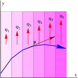
Figure 14.2 shows an example of what happens when a wave encounters a series of parallel slabs with increasing values of \(Q\). The \(y \) component of the wave vector doesn’t change as the wave crosses each of the interfaces between slabs, for reasons discussed above. Hence, \(\Pi_{y}=\hbar k_{y}\) doesn’t change either, which means that \(d \Pi_{y} d x=0\). The \(y \) component of kinetic momentum, \(p_{y}=\Pi_{y}-Q_{y},\), must therefore decrease as \(Q\) _y increases, as illustrated in figure 14.2.

Figure 14.3: A moving particle and a stationary pattern of potential momentum \(Q\) must be equivalent to a stationary particle and a moving pattern of potential momentum according to the principle of relativity.

Newton’s second law tells us that the \(y\) component of the force on the particle associated with the wave is just the time derivative of the \(y\) component of the kinetic momentum:

\[F_{y}=\frac{d p_{y}}{d t}=\frac{d p_{y}}{d x} \frac{d x}{d t}=\frac{d p_{y}}{d x} u_{x}=-\frac{d Q_{y}}{d x} u_{x}\label{14.14}\]

In the last step of this equation we used the fact that \(d \Pi_{y} / d x=0 .\).

The \(x \) component of the force can be obtained by similar reasoning, using the additional information that the speed, and hence the magnitude of the kinetic momentum, \(p^{2}=p_{x}^{2}+p_{y}^{2}\), doesn’t change under the influence of the potential momentum:

\[F_{x}=\frac{d p_{x}}{d t}=\frac{d p_{x}}{d x} \frac{d x}{d t}=-\frac{p_{y}}{\left(p^{2}-p_{y}^{2}\right)^{1 / 2}} \frac{d p_{y}}{d x} u_{x}=\frac{p_{y}}{p_{x}} \frac{d Q_{y}}{d x} u_{x}=\frac{d Q_{y}}{d x} u_{y} .\label{14.15}\]

Aside from assuming that \(p^{2}=\text { constant } \text { , }\), we have used the relationships \(p_{x}=\left(p^{2}-p_{y}^{2}\right)^{1 / 2} \text { and } p_{y} / p_{x}=u_{y} / u_{x}\). Equations (\ref{14.14}) and (\ref{14.15}) constitute a special case of equations (\ref{14.12}) and (\ref{14.13}) which is valid when \(Q\) points in the \(y\) direction and is a function only of \(x\).

Time-Varying Potential Momentum

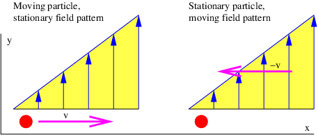
The necessity for the term \(-\partial \mathbf{Q} / \partial t\) in equation (\ref{14.12}) is easily understood from the following argument, which is illustrated in figure 14.3. The example in the previous section showed that a particle moving in the \(+x\) direction with velocity \(\mathrm{u}_{\mathrm{x}}\) through a field of increasing \(\mathrm{Q}_{\mathrm{y}}\) (left panel of figure 14.3) experiences a force in the -y direction equal to \(F_{y}=-\left(d Q_{y} / d x\right) u_{x}\). However, viewing this same process from a reference frame in which the particle is stationary (right panel of this figure), we see that the potential momentum at the position of the particle increases with time at the rate \(\mathrm{dQ}_{\mathrm{y}} / \mathrm{dt} \text { . }\). The particle is not moving in this reference frame, so the term \(\mathbf{v} \times \mathbf{P}=0\). However, the stationary particle must still experience the above force in this reference frame in order to satisfy the principle of relativity.

Noting that \(\mathrm{dQ}_{y} / \mathrm{dt}=\left(\mathrm{dQ}_{\mathrm{y}} / \mathrm{dx}\right) \mathrm{u}_{\mathrm{x}}\), we see that equation (\ref{14.12}) provides this force via the term \(-\partial \mathbf{Q} / \mathrm{d} \mathrm{t}\) in the reference frame moving with the particle. Thus, the time derivative term in equation (\ref{14.12}) is needed to maintain the principle of relativity; the same force occurs in the two different reference frames but originates from the term \(\mathbf{v} \times \mathbf{P}\) in the original reference frame and the term \(-\partial \mathbf{Q} / \partial \mathrm{t}\) in the frame moving with the particle.

Arguments similar to these were actually made by Einstein in his original 1905 paper on relativity.