23.1: States of a Brick

Figure 23.1: “Inner-spring mattress” model of the atoms in a solid body. Interatomic forces act like miniature springs connecting the atoms. As a result the whole system oscillates like a bunch of harmonic oscillators.

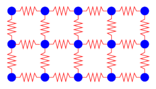
In this section we demonstrate the above assertions by making a crude model of the quantum mechanical states of a brick. We approximate the atoms of the brick as a collection of harmonic oscillators, three oscillators per atom, since each atom can oscillate in three dimensions under the influence of interatomic forces (see figure 23.1). For simplicity we assume that all of the oscillators have the same classical oscillation frequency, \(\omega_{0}\), so that the energy of each oscillator is given by

\[E_{n}=(n+1 / 2) \hbar \omega_{0} \equiv(n+1 / 2) E_{0}, \quad n=0,1,2, \ldots\label{23.1}\]

as reported in chapter 12. This assumption is a rather poor approximation to the behavior of a solid body when the total amount of internal energy is so small that many of the harmonic oscillators are in their ground state. However, it is adequate for situations in which the energy per oscillator is several times the ground state oscillator energy.

We further assume that each oscillator is weakly coupled to its neighbor. This allows a slow transfer of energy between oscillators without appreciably affecting the energy levels of each oscillator.

Figure 23.2: Diagrams for counting states of systems of two (left panel) and three (right panel) harmonic oscillators with the same classical oscillation frequency.

The next step is to calculate the number of states of a system of harmonic oscillators for which the total energy is less than some maximum value E. This calculation is easy for a system consisting of a single oscillator. From equation (\ref{23.1}) we infer that the number of states, \(\mathcal{N}\) of one oscillator with energy less than E is

\[\mathcal{N}=E / E_{0} \quad \text { (one oscillator) }\label{23.2}\]

since the states are evenly spaced in energy with spacing \(\mathrm{E}_{0}\).

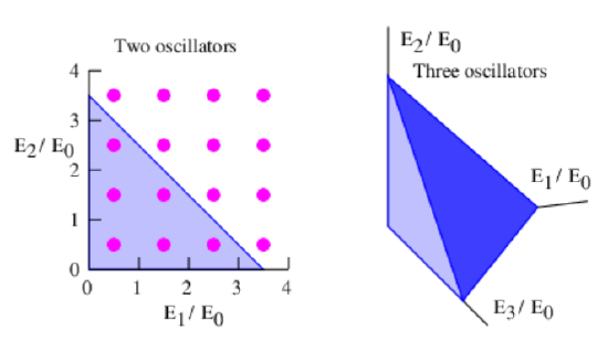
The calculation for a system of two oscillators is slightly more complicated. The dots in the left panel of figure 23.2 show the states available to a two oscillator system. Each dot corresponds to a unique pair of values of the quantum numbers n₁ and n₂ for the two oscillators. The total energy of the two oscillators together is \(\mathrm{E}_{\text {total }}=\mathrm{E}_{1}+\mathrm{E}_{2}=\left(\mathrm{n}_{1}+\mathrm{n}_{2}+1\right) \mathrm{E}_{0}\).

The line defined by the equation \(E / E_{0}=E_{1} / E_{0}+E_{2} / E_{0}\) is illustrated by the hypotenuse of the shaded triangle in the left panel of figure 23.2. The number of states with total energy less than E is obtained by simply counting the dots inside this triangle. An easy way to do this “counting” is to note that there is one dot per unit area in the plot, so that the number of dots approximately equals the area of the triangle:

\[\mathcal{N}=\frac{1}{2}\left(\frac{E}{E_{0}}\right)^{2} \quad \text { (two oscillators) }\label{23.3}\]

For a system of three oscillators the possible states of the system form a cubical grid in a three-dimensional space with axes \(\mathrm{E}_{1} / \mathrm{E}_{0}, \mathrm{E}_{2} / \mathrm{E}_{0,} \text { and } \mathrm{E}_{3} / \mathrm{E}_{0}\), as shown in the right panel of figure 23.2. The dots representing the states are omitted for clarity, but one state per unit volume exists in this space. The dark-shaded oblique triangle is the surface of constant total energy \(E\) defined by the equation \(\mathrm{E}_{1} / \mathrm{E}_{0}+\mathrm{E}_{2} / \mathrm{E}_{0}+\mathrm{E}_{3} / \mathrm{E}_{0}=\mathrm{E} / \mathrm{E}_{0}\), so the volume of the tetrahedron formed by this surface and the coordinate axis planes equals the number of states with energy less than E. This volume is computed as the area of the base of the tetrahedron, \(\left(\mathrm{E} / \mathrm{E}_{0}\right)^{2} / 2\), times its height, E ∕ E ₀, times 1 ∕ 3. We get

\[\mathcal{N}=\frac{1}{2 \cdot 3}\left(\frac{E}{E_{0}}\right)^{3} \quad \text { (three oscillators). }\label{23.4}\]

There is a pattern here. We infer that there are

\[\mathcal{N}(E)=\frac{1}{1 \cdot 2 \cdot 3 \ldots N}\left(\frac{E}{E_{0}}\right)^{N}=\frac{1}{N !}\left(\frac{E}{E_{0}}\right)^{N} \quad(N \text { oscillators })\label{23.5}\]

states available to N oscillators with total energy less than E. The notation N! is shorthand for 1 ⋅ 2 ⋅ 3…N and is pronounced “N factorial”.

Let us summarize what we have accomplished. \(\mathcal{N}_{(E)}\) is the number of states of a system of harmonic oscillators, taken together, with total energy less than E. What we need is an estimate of the number of states between two energy limits, say E and \(E+\Delta E \text { . }\). This is easily obtained from \(\mathcal{N}_{(E)}\) as follows: \(\mathcal{N}_{(E)}\)is the number of states with energy less than E, while \(\mathcal{N}(E+\Delta E)\) is the number of states with energy less than \(E+\Delta E \text { . }\). We can obtain the number of states with energies between E and \(E+\Delta E \text { . }\) by subtracting these two quantities:

\[\Delta \mathcal{N}=\mathcal{N}(E+\Delta E)-\mathcal{N}(E)=\frac{\mathcal{N}(E+\Delta E)-\mathcal{N}(E)}{\Delta E} \Delta E \approx \frac{\partial \mathcal{N}}{\partial E} \Delta E\label{23.6}\]

For N harmonic oscillators we find that

\[\Delta \mathcal{N}=\frac{N}{N !} \frac{E^{N-1}}{E_{0}^{N}} \Delta E=\frac{1}{(N-1) !}\left(\frac{E}{E_{0}}\right)^{N-1} \frac{\Delta E}{E_{0}}\label{23.7}\]

\[\begin{equation}
\begin{array}{rrr}
N & \Delta \mathcal{N}(r=5) & \Delta \mathcal{N}(r=10) \\
1 & 1 & 1 \\
2 & 5 & 10 \\
3 & 50 & 200 \\
4 & 563 & 4500 \\
5 & 6667 & 106667 \\
6 & 81381 & 2604167 \\
7 & 1012500 & 64800000 \\
8 & 12765734 & 1634013889 \\
9 & 162539683 & 41610158730 \\
10 & 2085209002 & 1067627008928 \\
11 & 26911444555 & 27557319223986 \\
12 & 349006782021 & 714765889577822
\end{array}
\end{equation}\]

Table 23.1: Number of states \(\Delta \mathcal{N}\) available to \(N\) identical harmonic oscillators between energies \(E\) and \(E+\Delta E\), where \(E=r N E_{0}\) and where we have chosen \(\Delta \mathrm{E}=\mathrm{E}_{0}\). Results are shown for two different values of \(r\).

Table 23.1 shows the number of states of a system of a small number of harmonic oscillators with energy between \(E\) and \(E+\Delta E\) where we have chosen \(\Delta \mathrm{E}=\mathrm{E}_{0}\). Results are shown for systems up to N = 12 (i. e., “microbricks” with up to 4 atoms, each with 3 modes of oscillation). The quantity r is defined to be the average value of the quantum number n of all the harmonic oscillators in the system; \(r=E /\left(\mathrm{NE}_{0}\right)\). Thus, \(\mathrm{r} \mathrm{E}_{0}\) is the average energy per oscillator. Recall that our calculation is only valid if \(r\) is appreciably greater than one. The number of available states is computed for r = 5 and 10.

We see that a few atoms considered jointly have an astonishingly large number of possible states. For instance, a system of 4 atoms (i. e., 12 oscillators) with r = 5 has about 3.5 × 10¹¹ states. Suppose we now confine this energy to only 2 of the atoms or 6 oscillators. In this case r doubles to a value of 10 since the same amount of internal energy is now spread among half the number of oscillators. Table 23.1 shows that this reduced system has only about 2.6 × 10⁶ states. The probability of having all of the energy of the 4 atom system in these 2 atoms is the ratio of the number of states in the 2 atom case to the total number of possible states of the 4 atom system, or 2.6 × 10⁶∕3.5 × 10¹¹ = 7.4 × 10^-6. This is a rather small number, which means that it is rare to find the system with all internal energy concentrated in two atoms.

We now determine how the number of states available to a system of harmonic oscillators behaves for a very large number of oscillators such as might be found in a real brick. Values of \(\Delta \mathcal{N}\) become so large in this case that it is useful to work in terms of the natural logarithm of \(\Delta \mathcal{N}\). For large N we can safely approximate \(\mathrm{N}-1 \text { by } \mathrm{N} \text { . }\) Using the properties of logarithms, we get

\[\begin{equation}
\begin{aligned}
\ln (\Delta \mathcal{N}) &=\ln \left(\frac{\left(E / E_{0}\right)^{N-1}}{(N-1) !} \frac{\Delta E}{E_{0}}\right) \\
& \approx \ln \left(\frac{\left(E / E_{0}\right)^{N}}{N !} \frac{\Delta E}{E_{0}}\right) \\
&=N \ln \left(E / E_{0}\right)-\ln (N !)+\ln \left(\Delta E / E_{0}\right) .
\end{aligned}
\end{equation}\label{23.8}\]

A useful mathematical result for large N is the Stirling approximation.

\[\ln (N !) \approx N \ln (N)-N \quad \text { (Stirling approximation) }\label{23.9}\]

Substituting this into equation (\ref{23.8}), using the fact that \(N \ln \left(E / E_{0}\right)-N \ln N=N \ln \left[E /\left(N E_{0}\right)\right]\), and rearranging results in

\[\ln (\Delta \mathcal{N})=N\left[\ln \left(\frac{E}{N E_{0}}\right)+1\right]+\ln \left(\frac{\Delta E}{E_{0}}\right) \quad(N \text { oscillators }) .\label{23.10}\]

We now return to the original question, which we state in this form: What fraction of the states of a brick corresponds to the special situation with all of the internal energy in half of the brick? A real brick has of order 3 × 10²⁵ atoms or about N = 10²⁶ oscillators. Half of the brick thus has N′ = 5 × 10²⁵ oscillators. If, as before, we assume that r = 5 when the internal energy is distributed throughout the brick, then we have r′ = 10 when all the energy is in half of the brick. Therefore the logarithm of the total number of available states is \(\ln (\Delta \mathcal{N})=N[\ln (r)+1]+\ln \left(\Delta E/E_{0}\right)\), while the logarithm of the number of states available when all the energy is in half of the brick is \(\ln \left(\Delta \mathcal{N}^{\prime}\right)=N^{\prime}\left[\ln \left(r^{\prime}\right)+1\right]+\ln \left(\Delta E /E_{0}\right)\). Putting in the numbers, we find that the probability of finding all the energy in half of the brick is

\[\begin{equation}
\begin{aligned}
\Delta \mathcal{N}^{\prime} / \Delta \mathcal{N}=& \exp \left[\ln \left(\Delta \mathcal{N}^{\prime}\right)-\ln (\Delta \mathcal{N})\right] \\
=& \exp \left[N^{\prime} \ln \left(r^{\prime}\right)+N^{\prime}+\ln \left(\Delta E / E_{0}\right)\right.\\
&\left.-N \ln (r)-N-\ln \left(\Delta E / E_{0}\right)\right] \\
=& \exp (-0.96 N)=\exp \left(-9.6 \times 10^{25}\right)=10^{-4.2 \times 10^{25}}
\end{aligned}
\end{equation}\label{23.11}\]

This probability is extremely small, and is zero for all practical purposes.

Notice that \(\Delta \mathrm{E}\), which we haven’t specified, cancels out. This typically happens in the theory when measurable quantities are calculated, and it shows that the actual value of \(\Delta \mathrm{E}\) isn’t important. Furthermore, for very large values of N typical of normal bricks, the term in equation (\ref{23.10}) containing \(\Delta \mathrm{E}\) is always negligible for any reasonable values of \(\Delta \mathrm{E}\). We therefore drop it in future calculations.

The variable \(\ln (\Delta \mathcal{N})\) is proportional to a quantity that we call the entropy, \(S\). The actual relationship is

\[S=k_{B} \ln (\Delta \mathcal{N}) \quad(\text { definition of entropy })\label{23.12}\]

where k_B = 1.38 × 10^-23 J K^-1 is called Boltzmann’s constant. Ludwig Boltzmann was a 19th century Austrian physicist who played a pivotal role in the development of the concept of entropy. The entropy of a brick containing N oscillators is therefore

\[S=N k_{B}\left[\ln \left(\frac{E}{N E_{0}}\right)+1\right] \quad(\text { entropy of } N \text { oscillators })\label{23.13}\]

As with the speed of light and Planck’s constant, Boltzmann’s constant is not really needed for a complete development of statistical mechanics. Its only role is to convert entropy and related quantities to everyday units. The conventional dimensions of entropy are thus the same as those of Boltzmann’s constant, or energy divided by temperature. However, more fundamentally, we consider entropy (without Boltzmann’s constant) to be a dimensionless quantity since it is just the logarithm of the number of available states.