8.6: Motion in Two and Three Dimensions

When a matter wave moves through a region of variable potential energy in one dimension, only the wavenumber changes. In two or three dimensions, the wave vector can change in both direction and magnitude. This complicates the calculation of particle movement. However, we already have an example of how to handle this situation, namely, the refraction of light. In that case Snell’s law tells us how the direction of the wave vector changes, while the dispersion relation combined with the constancy of the frequency gives us information about the change in the magnitude of the wave vector. For matter waves a similar procedure works, though the details are different, because we seek the consequences of a change in potential energy rather than a change in the index of refraction.

Figure 8.2: Refraction of a matter wave by a discontinuity in potential energy. The component of the wave vector parallel to the discontinuity, \(\mathrm{k}_{\mathrm{y}}\), doesn’t change, so \(\mathrm{k}_{1 \mathrm{y}}=\mathrm{k}_{2 \mathrm{y}}\).

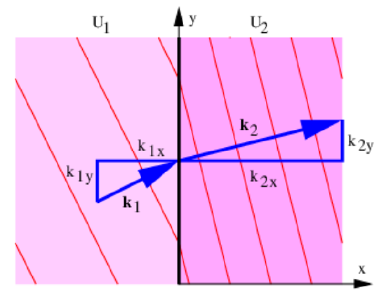
Figure 8.2 illustrates the refraction of matter waves at a discontinuity in the potential energy. Let us suppose that the discontinuity occurs at \(x=0\). If the matter wave to the left of the discontinuity is \(\Psi_{1}=\sin \left(\mathrm{k}_{1 \mathrm{x}} \mathrm{x}+\mathrm{k}_{1 \mathrm{y}} \mathrm{y}-\omega_{1} \mathrm{t}\right)\) and to the right is \(\Psi_{2}=\sin \left(\mathrm{k}_{2 \mathrm{x}} \mathrm{x}+\mathrm{k}_{2 \mathrm{y}} \mathrm{y}-\omega_{2} \mathrm{t}\right)\), then the wavefronts of the waves will match across the discontinuity for all time only if \(\omega_{1}=\omega_{2} \equiv \omega \text { and } \mathrm{k}_{1 \mathrm{y}}=\mathrm{k}_{2 \mathrm{y}} \equiv \mathrm{k}_{\mathrm{y}}\). We are already familiar with the first condition from the one-dimensional problem, so the only new ingredient is the constancy of the y component of the wave vector.

In two dimensions the momentum is a vector:\(\boldsymbol{\Pi}=\mathrm{mu} \text { when }|\mathbf{u}| \ll \mathrm{c}\), where u is the particle velocity. Furthermore, the kinetic energy is \(K=m|\mathbf{u}|^{2} / 2=|\mathbf{\Pi}|^{2} /(2 m)=\left(\Pi_{x}{ }^{2}+\Pi_{y}{ }^{2}\right) /(2 m)\). The relationship between kinetic, potential, and total energy is unchanged from the one-dimensional case, so we have

\[E=U+\left(\Pi_{x}^{2}+\Pi_{y}^{2}\right) /(2 m)=\text { constant. }\label{8.25}\]

The de Broglie relationship tells us that \(\boldsymbol{\Pi}=\hbar \mathbf{k}\), so the constancy of \(\mathrm{k}_{\mathrm{y}}\) across the discontinuity in U tells us that

\[\Pi_{y}=\text { constant }\label{8.26}\]

there

Figure 8.3: Trajectory of a wave packet through a variable potential energy, U(x), which decreases to the right.

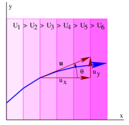
Let us now approximate a continuously variable U(x) by a series of steps of constant U oriented normal to the x axis. The above analysis can be applied at the jumps or discontinuities in U between steps, as illustrated in figure 8.3, with the result that equations (\ref{8.25}) and (\ref{8.26}) are valid across all discontinuities. If we now let the step width go to zero, these equations then become valid for U continuously variable in x.

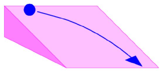
An example from classical mechanics of a problem of this type is a ball rolling down an inclined ramp with an initial velocity component across the ramp, as illustrated in figure 8.4. The potential energy decreases in the down ramp direction, resulting in a force down the ramp. This accelerates the ball in that direction, but leaves the component of momentum across the ramp unchanged.

Figure 8.4: Classical mechanics example of the problem illustrated in figure 8.3.

Using the procedure which we invoked before, we find the force components associated with U(x) in the x and y directions to be \(F_{x}=-d U / d x \text { and } F_{y}=0\). This generalizes to

\[\mathbf{F}=-\left(\frac{\partial U}{\partial x}, \frac{\partial U}{\partial y}, \frac{\partial U}{\partial z}\right) \quad \text { (3-D conservative force) }\label{8.27}\]

in the three-dimensional case where the orientation of constant U surfaces is arbitrary. It is also valid when U(x,y,z) is not limited to a simple ramp form, but takes on a completely arbitrary structure.

The definitions of work and power are slightly different in two and three dimensions. In particular, work is defined as

\[W=\mathbf{F} \cdot \Delta \mathbf{x}\label{8.28}\]

where Δx is now a vector displacement. The vector character of this expression yields an additional possibility over the one dimensional case, where the work is either positive or negative depending on the direction of Δx relative to F. If the force and the displacement of the object on which the force is acting are perpendicular to each other, the work done by the force is actually zero, even though the force and the displacement both have non-zero magnitudes. The power exhibits a similar change:

\[P=\mathbf{F} \cdot \mathbf{u}\label{8.29}\]

Thus the power is zero if an object’s velocity is normal to the force being exerted on it.

As in the one-dimensional case, the total work done on a particle equals the change in the particle’s kinetic energy. In addition, the work done by a conservative force equals minus the change in the associated potential energy.

Energy conservation by itself is somewhat less useful for solving problems in two and three dimensions than it is in one dimension. This is because knowing the kinetic energy at some point tells us only the magnitude of the velocity, not its direction. If conservation of energy fails to give us the information we need, then we must revert to Newton’s second law, as we did in the one-dimensional case. For instance, if an object of mass m has initial velocity \(\mathbf{u}_{0}=\left(\mathrm{u}_{0}, 0\right)\) at location \((x, z)=(0, h)\) and has the gravitational potential energy \(\mathrm{U}=\mathrm{mgz}\), then the force on the object is \(\mathbf{F}=(0,-\mathrm{mg})\). The acceleration is therefore \(\mathbf{a}=\mathbf{F} / \mathrm{m}=(0,-\mathrm{g})\). Since \(\mathbf{a}=\mathrm{d} \mathbf{u} / \mathrm{dt}=\mathrm{d}^{2} \mathbf{x} / \mathrm{dt}^{2}\) where \(\mathbf{x}=(\mathrm{x}, \mathrm{z})\) is the object’s position, we find that

\[\mathbf{u}=\left(C_{1},-g t+C_{2}\right) \quad \mathbf{x}=\left(C_{1} t+C_{3},-g t^{2} / 2+C_{2} t+C_{4}\right)\label{8.30}\]

where C₁, C₂, C₃, and C₄ are constants to be evaluated so that the solution reduces to the initial conditions at t = 0. The specified initial conditions tell us that C₁ = u₀, C₂ = 0, C₃ = 0, and C₄ = h in this case. From these results we can infer the position and velocity of the object at any time.