3.1: Kinematics

Kinematics

Concepts and Principles

If the forces acting on an object are not constant, then the acceleration of the object is not constant. To analyze the kinematics of an object undergoing non-constant acceleration requires the use of calculus. By re-examining our original definitions, valid in the limit of very small time intervals during which the acceleration is approximately constant, the relationships between position, velocity, and acceleration can be constructed in terms of the derivative.

 

Position

Let r(t) be the location of the object at every time, t, in the time interval of interest.

 

Velocity

Our original definition of velocity,

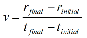
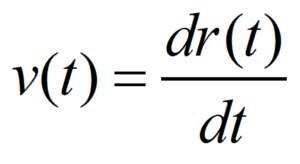
remains valid if the acceleration is constant. The acceleration will always be constant in the limit of infinitesimally small time intervals. By the fundamental definition of calculus, the above expression, in the limit of infinitesimally small time intervals, becomes the derivative of the position function. Thus, v(t), the velocity of the object at every time, t, is defined to be the derivative of the position function, r(t).

Acceleration

Our original definition of acceleration,

also remains valid only in the limit of infinitesimally small time intervals. By the fundamental definition of calculus, the above expression, in the limit of infinitesimally small time intervals, becomes the derivative of the velocity function. Thus, a(t), the acceleration of the object at every time, t, is defined to be the derivative of the velocity function, v(t).

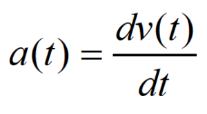
Thus, if the position of the object is known as a function of time, the velocity and acceleration functions can be constructed through differentiation of r(t). On the other hand, if the acceleration of the object is known as a function of time, the velocity and position functions can be constructed through anti-differentiation, or integration, of a(t).

An important distinction, however, is that when integrating a(t) to form v(t), an arbitrary constant will be introduced into the expression for v(t). This constant can often be determined from knowledge of the object’s velocity at some specific instant in time. Another integration, to form r(t), will introduce an additional arbitrary constant that can often be determined from knowledge of the object’s position at some specific instant in time.

In closing, please remember that the kinematic relations that have been used throughout this course were derived assuming a constant acceleration. If the acceleration is not constant, those relations are incorrect, and the correct kinematic relationships must be determined through direct integration and differentiation.

 

 

Analysis Tools

Using the Calculus

Investigate the scenario described below.

In a 100 m dash, detailed video analysis indicates that a particular sprinter’s speed can be modeled as a quadratic function of time at the beginning of the race, reaching 10.6 m/s in 2.70 s, and as a decreasing linear function of time for the remainder of the race. She finished the race in 12.6 seconds.

 

To analyze this situation, we should first carefully determine and define the sequence of events that take place. At each of these instants, let’s tabulate what we know about the motion.

Event 1: The race  begins     t1 = 0 s   r1 = 0 m   v1 = 0 m/s   a1 =

Event 2: She reaches 10.6 m/s     t2 = 2.7 s   r2 =   v2 = 10.6 m/s   a2 =

Event 3: She crosses the finish line     t3 = 12.6 s   r3 = 100 m   v3 =   a3 =

 

Since the acceleration is no longer necessarily constant between instants of interest, it is no longer useful to speak of a₁₂ or a₂₃. The acceleration, like the position and the velocity, is a function. What the table represents is the value of that function at specific instants of time.

Between event 1 and 2, the sprinter’s velocity can be modeled by a generic quadratic function of time^[1], or

Our job is to first determine (if possible) the arbitrary constants A and B, and then use this velocity function to find the position and acceleration functions.

Since the sprinter starts from rest, we can evaluate the function at t = 0 s and set the result equal to 0 m/s:

Since we also know the sprinter reaches a speed of 10.6 m/s in 2.7 s, we can evaluate the function at t = 2.7 s and set the result equal to 10.6 m/s:

Now that we know the two constants in the velocity function, we have a complete description of the sprinter’s speed during this time interval:

Once the velocity function is determined, we can differentiate to determine her acceleration function.

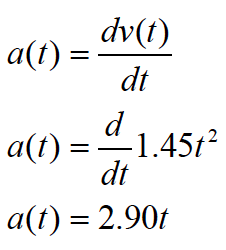
Evaluating this function at t = 0 s and t = 2.7 s yields a₁ = 0 m/s² and a₂ = 7.83 m/s².

 

We can also integrate to determine her position function.

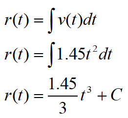
Since we know r = 0 m when t = 0 s, we can determine the integration constant:

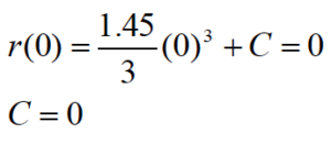
Therefore, the position of the sprinter is given by the function:

Evaluating this function at t = 0 s and t = 2.7 s yields r₁ = 0 m and r₂ = 9.51 m.

 

During the second portion of the race, when her speed is decreasing linearly, her acceleration is constant. Therefore, we can use the kinematic relations developed for constant acceleration, and her acceleration is simply a constant value, denoted a₂₃.

She crosses the finish line running at 7.68 m/s.

 

 

 

Another Example

Investigate the scenario described below.

A sports car can accelerate from rest to a speed of 40 m/s while traveling a distance of 200 m. Assume the acceleration of the car can be modeled as a decreasing linear function of time, with a maximum acceleration of 10.4 m/s².

 

Event 1: The car  begins from rest     t1 = 0 s   r1 = 0 m   v1 = 0 m/s   a1 = 10.4 m/s2

Event 2: The car reaches 40 m/s     t2 =   r2 = 200 m   v2 = 40 m/s   a2 =

 

Between event 1 and 2, the car’s acceleration can be modeled by a generic linear function of time, or

Since the acceleration is decreasing, the maximum value occurs at t = 0 s,

Since we don’t know the value of the acceleration at t₂, or even the value of t₂, we can’t determine A, and all we can currently say about the acceleration function is that it is given by:

Nonetheless, we can still integrate the acceleration to determine the velocity,

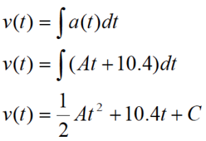
Since we know v = 0 m/s when t = 0 s, we can determine the integration constant:

We also know that v = 40 m/s at t₂, so:

This equation can’t be solved, since it involves two unknowns. However, if we can generate a second equation involving the same two unknowns, we can solve the two equations simultaneously. This second equation must involve the position function of the car:

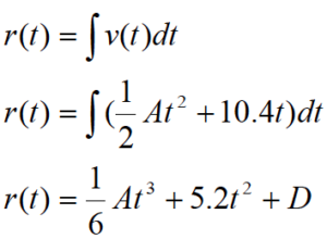
Since we know r = 0 when t = 0 s, we can determine the integration constant:

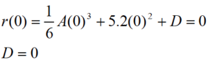
We also know that r = 200 m at t₂, so:

These two equations,

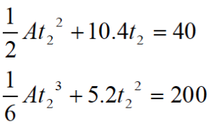
can be solved by substitution (or by using a solver). Solve the first equation for A, and substitute this expression into the second equation. This will result in a quadratic equation for t₂. The solution is t₂ = 7.57 s, the time for the car to reach 40 m/s. Plugging this value back into the original equations allows you to complete the description of the car’s motion.

 

Circular Motion

If the acceleration of an object is not constant, in either magnitude or direction, the development of a kinematic description necessitates the use of calculus. A very common class of motion, in which the acceleration is guaranteed to change in at least direction, is the motion of an object on a circular path. Let’s examine general circular motion in more detail before we attempt to describe a specific situation.

 

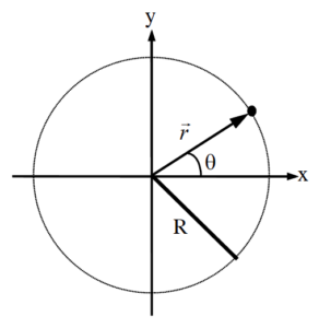The x- and y-position of the object moving along a circular path of radius R can always be described by the functions: 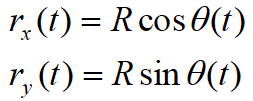assuming the origin of the coordinate system is placed at the center of the circle.

Defining angular position, angular velocity and angular acceleration

Angular Position

The function (t) specifies the angular position of the object, and is typically measured in radians. It specifies where, along the circle, the object is at every instant of time. For example, if (t) is a constant, the object doesn’t move. If (t) is a linear function of time, the object moves with constant velocity around the circle. If (t) is a more complex function, the object speeds up or slows down as it moves around the circle.

Angular Velocity

The rate at which (t) is changing, , is termed the angular velocity of the object, and denoted (t). ( is the lower-case Greek letter “omega”.^[2]) Since (t) is the rate at which the angular position is changing, it has units of rad/s.

Angular Acceleration

The rate at which (t) is changing, , is termed the angular acceleration of the object, and denoted (t). ( is the lower-case Greek letter “alpha”.) Since (t) is the rate at which the angular velocity is changing, it has units of rad/s².

 

Deriving relationships for velocity and acceleration

Now that we have the definitions of the angular quantities out of the way, let’s determine the velocity and acceleration of an object undergoing circular motion. I’ll begin by writing the position function in  notation, a common “short-hand” method of writing the x-, y-, and z- components of a vector all together. In this notation, the  simply stands for the x-component, the  for the y-component, and the  for any z-component. Hold onto your hat and try not to get lost in the calculus.

 

Position

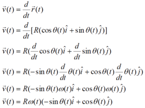
Velocity

Acceleration

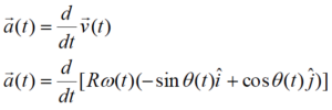
Remembering to use the chain rule for differentiation,

 

These relationships for velocity and acceleration look intimidating, but are actually rather simple. (You don’t have to believe me just yet …) The problem is that they are written using an awkward choice of coordinate system. In a previous Model, we used inclined coordinates for situations involving objects moving on an inclined surface. For an object moving in a circle, it’s almost as if the surface upon which the object moves is continually changing its angle of incline! Perhaps we should use a coordinate system in which the orientation of the system continually changes, always keeping one axis parallel and one axis perpendicular to the motion. This is exactly what we will do. This coordinate system is referred to as the polar coordinate system.

 
Polar Coordinates

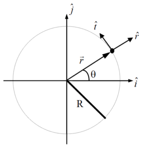
In the polar coordinate system, one axis (the radial axis, or ) is perpendicular to the surface of the circular path pointing radially away from the center, and the other axis (the tangential, or ) is parallel to the surface of the circular path pointing in the counterclockwise direction.

 

Notice that  is inclined by an angle q from the positive x-axis. Therefore, in terms of  and ; , on the other hand, is inclined by an angle  to the left of the positive y-axis. Therefore, in terms of  and ;

 

Now re-examine the relationships for position, velocity and acceleration.

 

Position

becomes^[3]

In component form this is:

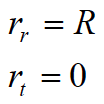
This means that the position of an object undergoing circular motion is only in the radial direction, and has a constant magnitude equal to the radius of the circle. Basically, the coordinate system is constructed so that the location of the object defines the radial direction.

 

Velocity

becomes

In component form this is:

This means that the velocity of an object undergoing circular motion is only in the tangential direction, and has a magnitude equal to the product of the radius and angular velocity. The only way an object can have a radial velocity is if the radius of its path changes, but that can’t happen for an object moving along a circular path. If the object moved along an elliptical path, for example, then it would have both tangential and radial velocities.

 

Acceleration

becomes

In component form this is:

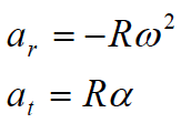
The acceleration of an object undergoing circular motion has two components. If the object is speeding up or slowing down, the angular acceleration does not equal zero and there is an acceleration component in the tangential direction. The magnitude of the tangential acceleration is equal to the product of the radius and angular acceleration.

However, even if the object is moving at constant speed, there is an acceleration component in the negative radial direction, i.e., pointing toward the center of the circle. By virtue of traveling in a circle, the velocity vector of an object continually changes its orientation. This change in orientation is directed toward the center of the circle. Draw a motion diagram and convince yourself of this fact!

The magnitude of the radial acceleration is equal to the product of the radius and the square of the angular velocity.

 

The Kinematics of Circular Motion

Let’s try out our new tools by examining the following scenario.

An automobile enters a U-turn of constant radius of curvature 95 m. The car enters the U-turn traveling at 33 m/s north and exits at 22 m/s south. Assume the speed of the car can be modeled as a quadratic function of time.

 

To analyze this situation, we should first carefully determine and define the sequence of events that take place. At each of these events we will tabulate the position, velocity and acceleration in polar coordinates as well as the angular position, angular velocity, and angular acceleration.

Notice that the position of the car is strictly in the radial direction and the velocity of the car is strictly in the tangential direction. It is impossible, for an object moving along a circular path, to have a non-zero tangential position or radial velocity.

Also notice that since the car completely reverses its direction of travel, it must have traveled halfway around a circular path. Thus, ₂ =  rad.

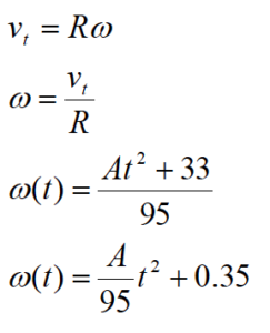
We can quickly determine the angular velocity of the car at the two events by using the relationship:

With R = 95 m, the angular velocity of the car as it enters the turn is 0.35 rad/s, and as it exits the turn, 0.23 rad/s.

 

Between event 1 and 2, the car’s speed can be modeled by a generic quadratic function of time, or

Since the car enters the turn at 33 m/s, we can evaluate the function at t = 0 s and set the result equal to 33 m/s:

The car exits the turn at 22 m/s, but since we don’t know the value of t₂ we can’t determine A. We do know, however, that:

If we can determine another equation involving A and t₂ we can solve these two equations simultaneously.

 

The only other important piece of information regarding the motion is that ₂ = . To make use of that information, we must “convert” our velocity equation into an angular velocity () equation and then integrate the resulting equation into an equation for . To determine the angular velocity function,

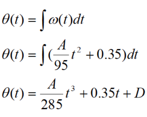
The angular position () is the integral of the angular velocity,

 

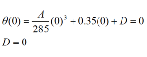
Since we know  = 0 when t = 0 s, we can determine the integration constant:

We also know that  =  at t₂, so:

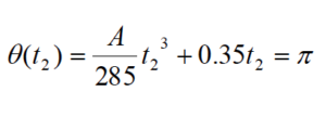
These two equations,

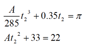
can be solved by substitution (or by using a solver). Solve the second equation for A, and substitute this expression into the first equation. You can solve the resulting equation for t₂. The solution is t₂ = 10.0 s, the time for the car to complete the turn. Plugging this value back into the original equation allows you to determine A = -0.11.

 

Once you know A, you can complete the rest of the motion table. For example, since

We can now determine angular acceleration,

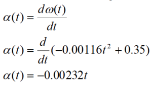
radial acceleration,

and tangential acceleration.

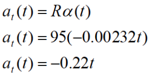
Each of these functions could be evaluated at t₁ = 0 s and t₂ = 10.0 s to complete the table.

 

 

Activities

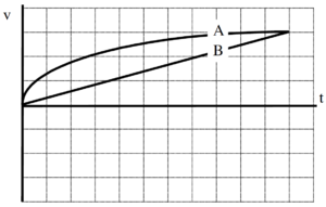
In a drag race, two cars begin from rest at the starting line and move according to the velocity vs. time graph below. Construct the position and acceleration vs. time graphs for each car.

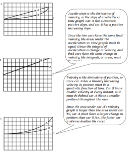
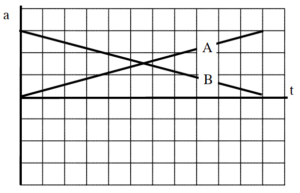
In a drag race, two cars begin from rest at the starting line and move according to the given kinematic graph. Construct the other two kinematic graphs for each car.

 

a.

b.

 

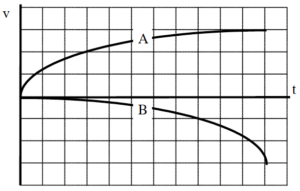
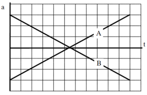
In a strange type of race, two cars begin from rest at the starting line and move according to the given kinematic graph. Construct the other two kinematic graphs for each car.

 

a.

b.

 

Below are velocity vs. time graphs for six different objects.

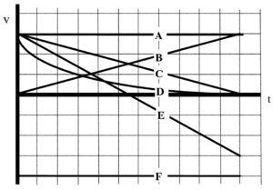
Rank these objects on the basis of their change in position during the time interval shown.

 

Largest Positive  1. _____ 2. _____ 3. _____ 4. _____ 5. _____ 6. _____ Largest Negative

 

_____ The ranking cannot be determined based on the information provided.

 

Explain the reason for your ranking:

 

 

 

 

Rank these objects on the basis of their change in acceleration during the time interval shown.

 

Largest Positive  1. _____ 2. _____ 3. _____ 4. _____ 5. _____ 6. _____ Largest Negative

 

_____ The ranking cannot be determined based on the information provided.

 

Explain the reason for your ranking:

 

 

 

 

 

Below are acceleration vs. time graphs for six different cars. All six cars begin a race at rest at the starting line.

 

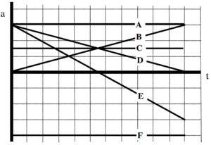
Rank these cars on the basis of their final velocity at the end of the time interval shown.

 

Largest Positive  1. _____ 2. _____ 3. _____ 4. _____ 5. _____ 6. _____ Largest Negative

 

_____ The ranking cannot be determined based on the information provided.

 

Explain the reason for your ranking:

 

 

 

 

Rank these cars on the basis of their final position at the end of the time interval shown.

 

Largest Positive  1. _____ 2. _____ 3. _____ 4. _____ 5. _____ 6. _____ Largest Negative

 

_____ The ranking cannot be determined based on the information provided.

 

Explain the reason for your ranking:

 

 

 

 

Construct motion diagrams for the motions described below.

 

A satellite has been programmed to circle a stationary space station at a radius of 10 km and a constant angular speed of 0.02 rad/s.

 

A rider on a merry-go-round, 3 m from the axis, is traveling at 4 m/s. The merry-go-round slows, and the rider reaches a speed of 0.5 m/s in 11 seconds.

 

In a device built to acclimate astronauts to large accelerations, astronauts are strapped into a pod that is swung in a 6 m radius circle at high speed. The linear speed of the pod is increased from rest to a speed of 17 m/s in a time interval of 25 seconds.

 

Sketch position, velocity, and acceleration vs. time graphs for one complete cycle of a rider on a merry-go-round turning at constant angular speed. Set the origin of the coordinate system at the center of the merry-go-round.

 

Sketch the x- and y-components of this motion separately.

 

Sketch the r- and t-components of this motion separately.

 

 

Sketch position, velocity, and acceleration vs. time graphs for one complete cycle of a rider on a Ferris wheel as it increases its angular speed from rest. Set the origin of the coordinate system at the center of the Ferris wheel.

 

Sketch the x- and y-components of this motion separately.

 

Sketch the r- and t-components of this motion separately.

 

 

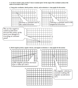
A car drives around a semi-circular U-turn at constant speed. Set the origin of the coordinate system at the center-of-curvature of the U-turn.

 

Using polar coordinates, sketch position, velocity, and acceleration vs. time graphs for this motion.

 

Sketch angular position, angular velocity, and angular acceleration vs. time graphs for this motion.

 

 

 

A car drives around a semi-circular U-turn at decreasing speed. Set the origin of the coordinate system at the center-of-curvature of the U-turn.

 

Using polar coordinates, sketch position, velocity, and acceleration vs. time graphs for this motion.

 

Sketch angular position, angular velocity, and angular acceleration vs. time graphs for this motion.

 

 

An artificial satellite circles a space station at constant speed. The satellite passes through the six labeled points. For all questions below, use the indicated coordinate system.

 

 

Rank the x-velocity of the satellite at each of the labeled points.

 

Largest Positive  1. _____ 2. _____ 3. _____ 4. _____ 5. _____ 6. _____ Largest Negative

 

_____ The ranking cannot be determined based on the information provided.

 

 

Rank the y-velocity of the satellite at each of the labeled points.

 

Largest Positive  1. _____ 2. _____ 3. _____ 4. _____ 5. _____ 6. _____ Largest Negative

 

_____ The ranking cannot be determined based on the information provided.

 

 

Rank the radial velocity of the satellite at each of the labeled points.

 

Largest Positive  1. _____ 2. _____ 3. _____ 4. _____ 5. _____ 6. _____ Largest Negative

 

_____ The ranking cannot be determined based on the information provided.

 

 

Rank the tangential velocity of the satellite at each of the labeled points.

 

Largest Positive  1. _____ 2. _____ 3. _____ 4. _____ 5. _____ 6. _____ Largest Negative

 

_____ The ranking cannot be determined based on the information provided.

 

 

Rank the angular velocity of the satellite at each of the labeled points.

 

Largest Positive  1. _____ 2. _____ 3. _____ 4. _____ 5. _____ 6. _____ Largest Negative

 

_____ The ranking cannot be determined based on the information provided.

 

 

 

Six artificial satellites of identical mass circle a space station with constant period T. The satellites are located a distance R from the space station.

 

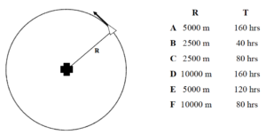
Rank these satellites on the basis of the magnitude of their angular velocity.

 

Largest  1. _____ 2. _____ 3. _____ 4. _____ 5. _____ 6. _____ Smallest

 

_____ The ranking cannot be determined based on the information provided.

 

Rank these satellites on the basis of the magnitude of their radial velocity.

 

Largest  1. _____ 2. _____ 3. _____ 4. _____ 5. _____ 6. _____ Smallest

 

_____ The ranking cannot be determined based on the information provided.

 

Rank these satellites on the basis of the magnitude of their tangential velocity.

 

Largest  1. _____ 2. _____ 3. _____ 4. _____ 5. _____ 6. _____ Smallest

 

_____ The ranking cannot be determined based on the information provided.

 

Explain the reason for your rankings:

 

 

 

Six artificial satellites of identical mass circle a space station at constant speed v. The satellites are located a distance R from the space station.

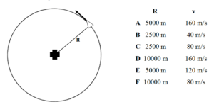
Rank these satellites on the basis of the magnitude of their angular acceleration.

 

Largest  1. _____ 2. _____ 3. _____ 4. _____ 5. _____ 6. _____ Smallest

 

_____ The ranking cannot be determined based on the information provided.

 

Rank these satellites on the basis of the magnitude of their radial acceleration.

 

Largest  1. _____ 2. _____ 3. _____ 4. _____ 5. _____ 6. _____ Smallest

 

_____ The ranking cannot be determined based on the information provided.

 

Rank these satellites on the basis of the magnitude of their tangential acceleration.

 

Largest  1. _____ 2. _____ 3. _____ 4. _____ 5. _____ 6. _____ Smallest

 

_____ The ranking cannot be determined based on the information provided.

 

Explain the reason for your rankings:

 

 

In a 100 m dash, detailed video analysis indicated that a particular sprinter’s speed can be modeled  as a quadratic function of time at the beginning of a race, reaching a speed of 12.1 m/s in 1.7 s, and then as a linear function of time for the remainder of the race. She finished the race in 10.6 seconds.

 

Motion Information

 

Event 1:     t1 =   r1 =   v1 =   a1 =

Event 2:     t2 =   r2 =   v2 =   a2 =

Event 3:     t3 =   r3 =   v3 =   a3 =

Mathematical Analysis[i]

 

 

In a 400 m race, detailed video analysis indicated that a particular sprinter’s speed can be modeled as a cubic function of time at the beginning of a race, reaching a speed of 8.5 m/s in 7.1 s, and as a linear function of time for the remainder of the race. She crossed the finish line traveling at 7.4 m/s.

 

Motion Information

 

Event 1:     t1 =   r1 =   v1 =   a1 =

Event 2:     t2 =   r2 =   v2 =   a2 =

Event 3:     t3 =   r3 =   v3 =   a3 =

Mathematical Analysis[ii]

 

 

 

 

Two cars, an Audi and a BMW, can accelerate from rest to a speed of 25 m/s in a time of 6.2 s. The velocity of the Audi increases as a linear function of time and the velocity of the BMW increases as a quadratic function of time.

 

Motion Graph                                                                           Motion Information

 

Audi Event 1:     t1 =   r1 =   v1 =   a1 =

Event 2:     t2 =   r2 =   v2 =   a2 =

BMW Event 1:     t1 =   r1 =   v1 =   a1 =

Event 2:     t2 =   r2 =   v2 =   a2 =

Question

Based only on the graph, which car travels a larger distance in 6.2 s? Explain.

 

 

 

 

Mathematical Analysis[iii]

 

 

Two cars, an Audi and a BMW, can accelerate from rest to a speed of 40 m/s after traveling a distance of 400 m. The velocity of the Audi increases as a linear function of time and the velocity of the BMW increases as a quadratic function of time.

 

Motion Graph                                                                           Motion Information

 

Audi Event 1:     t1 =   r1 =   v1 =   a1 =

Event 2:     t2 =   r2 =   v2 =   a2 =

BMW Event 1:     t1 =   r1 =   v1 =   a1 =

Event 2:     t2 =   r2 =   v2 =   a2 =

Question

Based only on the graph, which car will take longer to reach 40 m/s? Explain.

 

Mathematical Analysis[iv]

 

 

 

Two cars, an Audi and a BMW, accelerating from rest, can travel a distance of 400 m in 16.2 s. The velocity of the Audi increases as a linear function of time and the velocity of the BMW increases as a quadratic function of time.

 

Motion Graph                                                                           Motion Information

 

Audi Event 1:     t1 =   r1 =   v1 =   a1 =

Event 2:     t2 =   r2 =   v2 =   a2 =

BMW Event 1:     t1 =   r1 =   v1 =   a1 =

Event 2:     t2 =   r2 =   v2 =   a2 =

Question

Based only on the graph, which car is traveling faster at 16.2 s? Explain.

 

Mathematical Analysis[v]

 

 

 

Two cars, an Audi and a BMW, can accelerate from 15 m/s to 25 m/s in a time of 3.9 s. The velocity of the Audi increases as a linear function of time and the velocity of the BMW increases as a quadratic function of time.

 

Motion Graph                                                                           Motion Information

 

Audi Event 1:     t1 =   r1 =   v1 =   a1 =

Event 2:     t2 =   r2 =   v2 =   a2 =

BMW Event 1:     t1 =   r1 =   v1 =   a1 =

Event 2:     t2 =   r2 =   v2 =   a2 =

Question

Based only on the graph, which car travels a larger distance while accelerating? Explain.

 

Mathematical Analysis[vi]

 

 

Two cars, an Audi and a BMW, can slow from 35 m/s to 5 m/s over a distance of 70 m. The velocity of the Audi decreases as a linear function of time and the velocity of the BMW decreases as a quadratic function of time.

 

Motion Graph                                                                           Motion Information

 

Audi Event 1:     t1 =   r1 =   v1 =   a1 =

Event 2:     t2 =   r2 =   v2 =   a2 =

BMW Event 1:     t1 =   r1 =   v1 =   a1 =

Event 2:     t2 =   r2 =   v2 =   a2 =

Question

Based only on the graph, which car takes a longer time to slow to 5 m/s? Explain.

 

Mathematical Analysis[vii]

 

 

In a hypothetical universe, the acceleration of an object subject to the gravitational force field of an Earth-like planet decreases with the amount of time in seconds, t, spent in the field as

a = (9.8 m/s2) e -0.1 t

A ball is released from rest 100 m above the ground.

 

Motion Information 

Event 1: The ball is released.     t1 =   r1 =   v1 =   a1 =

Event 2: The ball hits the ground.     t2 =   r2 =   v2 =   a2 =

 

Mathematical Analysis[viii]

 

In a hypothetical universe, the acceleration of an object subject to the gravitational force field of an Earth-like planet decreases with the amount of time in seconds, t, spent in the field as

A ball is thrown vertically upward at 40 m/s.

 

Motion Information                                                                              

Event 1: The ball is released.     t1 =   r1 =   v1 =   a1 =

Event 2: The ball reaches its apex.     t2 =   r2 =   v2 =   a2 =

Event 3: The ball returns to your hand.     t3 =   r3 =   v3 =   a3 =

Mathematical Analysis[ix]

 

 

In a hypothetical universe, the acceleration of an object subject to the gravitational force field of an Earth-like planet increases with the amount of time in seconds, t, spent in the field as

a = (9.8 m/s2) (1 – e -0.1 t)

A ball is released from rest 100 m above the ground.

 

Motion Information

Event 1: The ball is released.     t1 =   r1 =   v1 =   a1 =

Event 2: The ball hits the ground.     t2 =   r2 =   v2 =   a2 =

 

Mathematical Analysis[x]

 

In a hypothetical universe, the acceleration of an object subject to the gravitational force field of an Earth-like planet increases with the amount of time in seconds, t, spent in the field as

a = (9.8 m/s2) (1 – e -0.1 t)

A ball is thrown vertically upward at 40 m/s.

 

Motion Information                                                                              

Event 1: The ball is released.     t1 =   r1 =   v1 =   a1 =

Event 2: The ball reaches its apex.     t2 =   r2 =   v2 =   a2 =

Event 3: The ball returns to your hand.     t3 =   r3 =   v3 =   a3 =

 

Mathematical Analysis[xi]  

 

A rider on a merry-go-round is traveling at a constant speed of 4.0 m/s, and completes three revolutions in 14 s.

 

Motion Information                                                                               Mathematical Analysis[xii]

Event 1:     t1 =   r1r = r1t = q1 =   v1r = v1t = w1 =   a1r = a1t = a1 =

Event 2:     t2 =   r2r = r2t = q2 =   v2r = v2t = w2 =   a2r = a2t = a2 =

 

 

 

A rider on a merry-go-round, 3.0 m from the axis, is traveling at 4.0 m/s. The merry-go-round slows to rest over three complete revolutions. The rider’s speed decreases as a linear function of time.

 

Motion Information                                                                               Mathematical Analysis[xiii]

 

Event 1:     t1 =   r1r = r1t = q1 =   v1r = v1t = w1 =   a1r = a1t = a1 =

Event 2:     t2 =   r2r = r2t = q2 =   v2r = v2t = w2 =   a2r = a2t = a2 =

 

 

A rider on a 15 m diameter Ferris wheel is initially at rest. The angular speed of the Ferris wheel is increased to 1.5 rad/s over a time interval of 3.5 s. The angular acceleration of the Ferris wheel increases from 0 rad/s2 as a square-root function of time.

 

Motion Information                                                                               Mathematical Analysis[xiv]

Event 1:     t1 =   r1r = r1t = q1 =   v1r = v1t = w1 =   a1r = a1t = a1 =

Event 2:     t2 =   r2r = r2t = q2 =   v2r = v2t = w2 =   a2r = a2t = a2 =

 

 

 

A rider on a 16 m diameter Ferris wheel is initially at traveling at 10 m/s. The Ferris wheel slows to rest over two complete revolutions. During the slow-down, the magnitude of the angular acceleration of the Ferris wheel decreases linearly from its maximum value to 0 rad/s2.

 

Motion Information                                                                               Mathematical Analysis[xv]

Event 1:     t1 =   r1r = r1t = q1 =   v1r = v1t = w1 =   a1r = a1t = a1 =

Event 2:     t2 =   r2r = r2t = q2 =   v2r = v2t = w2 =   a2r = a2t = a2 =

 

An automobile enters a constant 90 m radius of curvature turn traveling at 25 m/s north and exits the curve traveling at 35 m/s east. Assume the speed of the car can be modeled as a square-root function of time.

 

Motion Information                                                                               Mathematical Analysis[xvi]

Event 1:     t1 =   r1r = r1t = q1 =   v1r = v1t = w1 =   a1r = a1t = a1 =

Event 2:     t2 =   r2r = r2t = q2 =   v2r = v2t = w2 =   a2r = a2t = a2 =

 

 

 

 

 

An automobile enters a constant 90 m radius of curvature turn traveling at 25 m/s north and exits the curve traveling east. The car completes the turn in 5.4 s. Assume the speed of the car can be modeled as a quadratic function of time.

 

Motion Information                                                                               Mathematical Analysis[xvii]

Event 1:     t1 =   r1r = r1t = q1 =   v1r = v1t = w1 =   a1r = a1t = a1 =

Event 2:     t2 =   r2r = r2t = q2 =   v2r = v2t = w2 =   a2r = a2t = a2 =

 

 

 

In a device built to acclimate astronauts to large accelerations, astronauts are strapped into a pod that is swung in a 6.0 m radius circle at high speed. The angular speed of the pod is increased quadratically from rest to an angular speed of 2.8 rad/s in a time interval of 20 seconds. The device is then linearly slowed to rest over a time interval of 40 seconds.

 

Motion Information                                                                                                       Mathematical Analysis[xviii]

Event 1:     t1 =   r1r = r1t = q1 =   v1r = v1t = w1 =   a1r = a1t = a1 =

Event 2:     t2 =   r2r = r2t = q2 =   v2r = v2t = w2 =   a2r = a2t = a2 =

Event 3:     t3 =   r3r = r3t = q3 =   v3r = v3t = w3 =   a3r = a3t = a3 =

 

 

In a device built to acclimate astronauts to large accelerations, astronauts are strapped into a pod that is swung in a 6.0 m radius circle at high speed. The linear speed of the pod is increased quadratically from rest to a speed of 17 m/s after three complete revolutions of the pod. The device is then linearly slowed to rest over a time interval of 35 seconds.

 

Motion Information                                                                                                       Mathematical Analysis[xix]

Event 1:     t1 =   r1r = r1t = q1 =   v1r = v1t = w1 =   a1r = a1t = a1 =

Event 2:     t2 =   r2r = r2t = q2 =   v2r = v2t = w2 =   a2r = a2t = a2 =

Event 3:     t3 =   r3r = r3t = q3 =   v3r = v3t = w3 =   a3r = a3t = a3 =

[i] v3 = 8.83 m/s

[ii] t3 = 55.5 s

[iii] r2 bmw = 51.7 m

[iv] t2 bmw = 30 s

[v] v2 bmw = 74.1 m/s

[vi] r2 bmw = 71.5 m

[vii] t2 bmw = 2.8 s

[viii] t = 4.9 s

[ix] t3 = 11.6 s

[x] t2 = 9.3 s

[xi] t3 = 19.3 s

[xii] rr = 2.97 m

[xiii] t2 = 28.3 s

[xiv] q2 = 2.1 rad

[xv] t2 = 30.2 s

[xvi] t2 = 4.46 s

[xvii] v2 = 28.5 m/s

[xviii] q3 = 74.7 rad

[xix] q3 = 68.4 rad

http://www.compadre.org/IVV/vignettes/circularMotion.cfm

Homework 7 – Model 3: 25, 27, 32, 33, 34, 36, 37, 38, 47, 51.

---

1. When I say a “quadratic function of time”, I mean a function that only contains a term in which the time variable is squared (along with a time-independent constant). I don’t mean a polynomial of degree two, i.e., At² + Bt + C. This may or may not agree with the terminology you learned in math class. ↵
   
2. Call it “omega” don’t call it “double-you”. It will make you sound smarter. ↵
   
3. There’s always a bit of complaining regarding this formula. It looks like it says “r is equal to r times r” but these three “r’s” have completely different meanings. 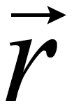 is the position of the object in space and has components in 2 (or more generally 3) directions. It can be expressed in any coordinate system. R is the magnitude of the position in polar coordinates.  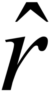is simply notation telling you that the position magnitude is measured radially away from the origin. ↵
   

CC licensed content, Original

• University Physics I Homework Assignments. Authored by: Mary Mohr. License: CC BY-NC-SA: Attribution-NonCommercial-ShareAlike