3.7: Adiabatic Processes for an Ideal Gas

Learning Objectives

By the end of this section, you will be able to:

• Define adiabatic expansion of an ideal gas
• Demonstrate the qualitative difference between adiabatic and isothermal expansions

When an ideal gas is compressed adiabatically \((Q = 0)\), work is done on it and its temperature increases; in an adiabatic expansion, the gas does work and its temperature drops. Adiabatic compressions actually occur in the cylinders of a car, where the compressions of the gas-air mixture take place so quickly that there is no time for the mixture to exchange heat with its environment. Nevertheless, because work is done on the mixture during the compression, its temperature does rise significantly. In fact, the temperature increases can be so large that the mixture can explode without the addition of a spark. Such explosions, since they are not timed, make a car run poorly—it usually “knocks.” Because ignition temperature rises with the octane of gasoline, one way to overcome this problem is to use a higher-octane gasoline.

Figure \(\PageIndex{1}\): The gas in the left chamber expands freely into the right chamber when the membrane is punctured.

Another interesting adiabatic process is the free expansion of a gas. Figure \(\PageIndex{1}\) shows a gas confined by a membrane to one side of a two-compartment, thermally insulated container. When the membrane is punctured, gas rushes into the empty side of the container, thereby expanding freely. Because the gas expands “against a vacuum” \((p = 0)\), it does no work, and because the vessel is thermally insulated, the expansion is adiabatic. With \(Q = 0\) and \(W = 0\) in the first law, \(\Delta E_{int} = 0\) so \(E_{int \, i} = E_{int \, f}\) for free expansion.

If the gas is ideal, the internal energy depends only on the temperature. Therefore, when an ideal gas expands freely, its temperature does not change; this is also called a Joule expansion.

Figure \(\PageIndex{2}\): When sand is removed from the piston one grain at a time, the gas expands adiabatically and quasi-statically in the insulated vessel.

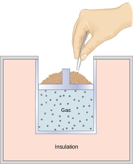
A quasi-static, adiabatic expansion of an ideal gas is represented in Figure \(\PageIndex{2}\), which shows an insulated cylinder that contains 1 mol of an ideal gas. The gas is made to expand quasi-statically by removing one grain of sand at a time from the top of the piston. When the gas expands by \(dV\), the change in its temperature is \(dT\). The work done by the gas in the expansion is \(dW = pdV\); \(dQ = 0\) because the cylinder is insulated; and the change in the internal energy of the gas is

\[dE_{int} = C_{V}ndT. \nonumber\]

Therefore, from the first law,

\[\begin{align*} C_{V}ndT &= 0 - pdV \\[4pt] &= -pdV \end{align*}\]

so

\[dT = -\dfrac{pdV}{C_{V}n}. \nonumber\]

Also, for 1 mol of an ideal gas,

[d(pV) = d(RnT), \nonumber\]

so

\[pdV + V \, dp = RndT \nonumber\]

and

\[dT = \dfrac{pdV + V \, dp}{Rn}.\nonumber\]

We now have two equations for \(dT\). Upon equating them, we find that

\[C_{V}n V dp + (C_{V}n + Rn)pdV = 0.\nonumber\]

Now, we divide this equation by \(npV\) and use \(C_p = C_V + R\). We are then left with

\[C_V \dfrac{dp}{p} + C_p\dfrac{dV}{V} = 0,\nonumber\]

which becomes

\[\dfrac{dp}{p} + \gamma\dfrac{dV}{V} = 0,\nonumber\]

where we define \(\gamma\) as the ratio of the molar heat capacities:

\[\gamma = \dfrac{C_p}{C_V}.\nonumber\]

Thus

\[\int \dfrac{dp}{p} + \gamma \int \dfrac{dV}{V} = 0\nonumber\]

and

\[ \ln \, p + \gamma ln \, V = constant.\nonumber\]

Finally, using \(\ln(A^x) = x \ln A\) and \(\ln \, AB = \ln \, A + \ln \, B\), we can write this in the form

\[pV^{\gamma} = constant. \label{eq10}\]

This equation is the condition that must be obeyed by an ideal gas in a quasi-static adiabatic process. For example, if an ideal gas makes a quasi-static adiabatic transition from a state with pressure and volume \(p_1\) and \(V_1\) to a state with \(p_2\) and \(V_2\), then it must be true that \(p_1V_1^{\gamma} = p_2V_2^{\gamma}\).

The adiabatic condition of Equation \ref{eq10} can be written in terms of other pairs of thermodynamic variables by combining it with the ideal gas law. In doing this, we find that

\[p^{1-\gamma}T^{\gamma} = constant\]

and

\[TV^{\gamma - 1} = constant.\]

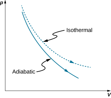
A reversible adiabatic expansion of an ideal gas is represented on the pV diagram of Figure \(\PageIndex{1}\). The slope of the curve at any point is

\[\dfrac{dp}{dV} = \dfrac{d}{dV}\left(\dfrac{constant}{V^{\gamma}}\right) = - \gamma \dfrac{p}{V}.\]

Figure \(\PageIndex{3}\): Quasi-static adiabatic and isothermal expansions of an ideal gas.

The dashed curve shown on this pV diagram represents an isothermal expansion where \(T\) (and therefore pV) is constant. The slope of this curve is useful when we consider the second law of thermodynamics in the next chapter. This slope is

\[\dfrac{dp}{dV} = \dfrac{d}{dV} \dfrac{nRT}{V} = - \dfrac{p}{V}.\]

Because \(\gamma >1\), the isothermal curve is not as steep as that for the adiabatic expansion.

Example \(\PageIndex{1}\): Compression of an Ideal Gas in an Automobile Engine

Gasoline vapor is injected into the cylinder of an automobile engine when the piston is in its expanded position. The temperature, pressure, and volume of the resulting gas-air mixture are \(20^oC\), \(1.00 \times 10^5 \, N/m^2\), and \(240 \, cm^3\), respectively. The mixture is then compressed adiabatically to a volume of \(40 \, cm^3\). Note that in the actual operation of an automobile engine, the compression is not quasi-static, although we are making that assumption here.

1. What are the pressure and temperature of the mixture after the compression?
2. How much work is done by the mixture during the compression?

Strategy

Because we are modeling the process as a quasi-static adiabatic compression of an ideal gas, we have \(pV^{\gamma} = constant\) and \(pV = nRT\). The work needed can then be evaluated with \(W = \int_{V_1}^{V_2} pdV\).

Solution

1. For an adiabatic compression we have \[p_2 = p_1\left(\dfrac{V_1}{V_2}\right)^{\gamma},\] so after the compression, the pressure of the mixture is \[p_2 = (1.00 \times 10^5 \, N/m^2)\left(\dfrac{240 \times 10^{-6}m^3}{40 \times 10^{-6}m^3}\right)^{1.40} = 1.23 \times 10^6 \, N/m^2.\] From the ideal gas law, the temperature of the mixture after the compression is \[\begin{align*}T_2 &= \left(\dfrac{p_2V_2}{p_1V_1}\right)T_1 \\[4pt] &= \dfrac{(1.23 \times 10^6 \, N/m^2)(40 \times 10^{-6} m^3)}{(1.00 \times 10^5 \, N/m^2)(240 \times 10^{-6} m^3)} \cdot 293 \, K \\[4pt] &= 600 \, K = 328^oC. \end{align*}\]
2. The work done by the mixture during the compression is \[W = \int_{V_1}^{V_2} pdV.\] With the adiabatic condition of Equation \ref{eq10}, we may write p as \(K/V^{\gamma}\), where \(K = p_1V_1^{\gamma} = p_2V_2^{\gamma}\). The work is therefore \[\begin{align*} W &= \int_{V_1}^{V_2} \dfrac{K}{V^{\gamma}} dV \\[4pt] &= \frac{K}{1 - \gamma}\left(\dfrac{1}{V_2^{\gamma -1}} - \dfrac{1}{V_1^{\gamma -1}}\right) \\[4pt] &= \dfrac{1}{1 - \gamma} \left(\dfrac{p_2V_2^{\gamma}}{V_2^{\gamma -1}} - \dfrac{p_1V_1^{\gamma}}{V_1^{\gamma -1}}\right) \\[4pt] &=\dfrac{1}{1 - \gamma}(p_2V_2 - p_1V_1) \\[4pt] &= \dfrac{1}{1 - 1.40}\left[(1.23 \times 10^6 \, N/m^2)(40 \times 10^{-6}m^3) - (1.00 \times 10^5 \, N/m^2)(240 \times 10^{-6}m^3)\right] \\[4pt] &= -63 \, J. \end{align*}\]

Significance

The negative sign on the work done indicates that the piston does work on the gas-air mixture. The engine would not work if the gas-air mixture did work on the piston.