12.5: Magnetic Field of a Current Loop

Learning Objectives

By the end of this section, you will be able to:

• Explain how the Biot-Savart law is used to determine the magnetic field due to a current in a loop of wire at a point along a line perpendicular to the plane of the loop.
• Determine the magnetic field of an arc of current.

The circular loop of Figure \(\PageIndex{1}\) has a radius R, carries a current I, and lies in the xz-plane. What is the magnetic field due to the current at an arbitrary point P along the axis of the loop?

Figure \(\PageIndex{1}\): Determining the magnetic field at point P along the axis of a current-carrying loop of wire.

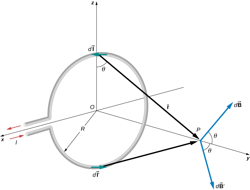
We can use the Biot-Savart law to find the magnetic field due to a current. We first consider arbitrary segments on opposite sides of the loop to qualitatively show by the vector results that the net magnetic field direction is along the central axis from the loop. From there, we can use the Biot-Savart law to derive the expression for magnetic field.

Let P be a distance y from the center of the loop. From the right-hand rule, the magnetic field \(d\vec{B}\) at P, produced by the current element \(I \, d\vec{l}\) is directed at an angle \(\theta\) above the y-axis as shown. Since \(d\vec{l}\) is parallel along the x-axis and \(\hat{r}\) is in the yz-plane, the two vectors are perpendicular, so we have

\[dB = \frac{\mu_0}{4\pi} \frac{I \, dl \, sin \, \pi/2}{r^2} = \frac{\mu_0}{4\pi} \frac{I \, dl}{y^2 + R^2} \label{12.13}\] where we have used \(r^2 = y^2 + R^2\).

Now consider the magnetic field \(d\vec{B}'\) due to the current element \(I \, d\vec{l}'\), which is directly opposite \(I \, d\vec{l}\) on the loop. The magnitude of \(d\vec{B}'\) is also given by Equation \ref{12.13}, but it is directed at an angle θ below the y-axis. The components of \(d\vec{B}\) and \(d\vec{B}'\) perpendicular to the y-axis therefore cancel, and in calculating the net magnetic field, only the components along the y-axis need to be considered. The components perpendicular to the axis of the loop sum to zero in pairs. Hence at point P:

\[\vec{B} = \hat{j} \int_{loop} dB \, cos \, \theta = \hat{j} \frac{\mu_0 I}{4\pi} \int_{loop}\frac{cos \, \theta \, dl}{y^2 + R^2}. \label{12.14}\]

For all elements \(d\vec{l}\) on the wire, y, R, and \(\theta\) are constant and are related by

\[cos \, \theta = \frac{R}{\sqrt{y^2 + R^2}}. \nonumber\]

Now from Equation \ref{12.14}, the magnetic field at P is

\[\vec{B} = \hat{j}\frac{\mu_0IR}{4\pi (y^2 + R^2)^{3/2}} \int_{loop}dl = \frac{\mu_0 IR^2}{2(y^2 + R^2)^{3/2}}\hat{j} \label{12.15}\] where we have used \(\int_{loop}dl = 2\pi R\). As discussed in the previous chapter, the closed current loop is a magnetic dipole of moment \(\vec{\mu} = I \, A\hat{n}\). For this example, \(A = \pi R^2\) and \(\hat{n} = \hat{j}\), so the magnetic field at P can also be written as

\[\vec{B} = \frac{\mu_0 \mu \hat{j}}{2\pi (y^2 + R^2)^{3/2}}. \label{12.16}\]

By setting \(y = 0\) in Equation \ref{12.16}, we obtain the magnetic field at the center of the loop:

Note

\[\vec{B} = \frac{\mu_0 I}{2R} \hat{j} \label{12.17}.\]

This equation becomes \(B = \mu_0 n I/(2R)\) for a flat coil of n loops per length. It can also be expressed as

\[\vec{B} = \frac{\mu_0\vec{\mu}}{2\pi R^3}. \label{12.18}\]

If we consider \(y >> R\) in Equation \ref{12.16}, the expression reduces to an expression known as the magnetic field from a dipole:

\[\vec{B} = \frac{\mu_0 \vec{\mu}}{2\pi y^3}. \label{12.19}\]

The calculation of the magnetic field due to the circular current loop at points off-axis requires rather complex mathematics, so we’ll just look at the results. The magnetic field lines are shaped as shown in Figure \(\PageIndex{2}\). Notice that one field line follows the axis of the loop. This is the field line we just found. Also, very close to the wire, the field lines are almost circular, like the lines of a long straight wire.

Figure \(\PageIndex{2}\): Sketch of the magnetic field lines of a circular current loop.

Magnetic Field between Two Loops

Two loops of wire carry the same current of 10 mA, but flow in opposite directions as seen in Figure \(\PageIndex{3}\). One loop is measured to have a radius of \(R = 50 \, cm\) while the other loop has a radius of \(2R = 100 \, cm\). The distance from the first loop to the point where the magnetic field is measured is 0.25 m, and the distance from that point to the second loop is 0.75 m. What is the magnitude of the net magnetic field at point P?

Figure \(\PageIndex{3}\): Two loops of different radii have the same current but flowing in opposite directions. The magnetic field at point P is measured to be zero.

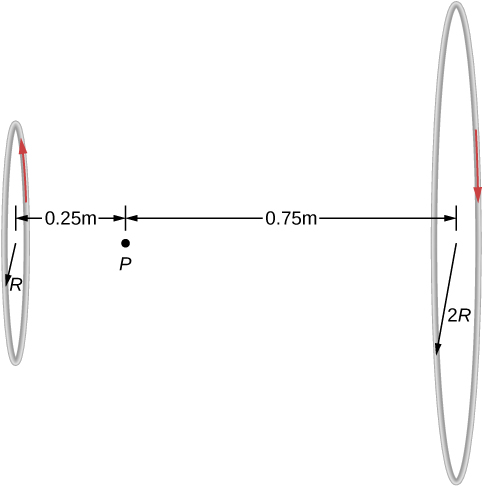
Strategy

The magnetic field at point P has been determined in Equation \ref{12.15}. Since the currents are flowing in opposite directions, the net magnetic field is the difference between the two fields generated by the coils. Using the given quantities in the problem, the net magnetic field is then calculated.

Solution

Solving for the net magnetic field using Equation \ref{12.15} and the given quantities in the problem yields

\[B = \frac{\mu_0 IR_1^2}{2(y_1^2 + R_1^2)^{3/2}} - \frac{\mu_0 IR_2^2}{2(y_2^2 + R_2^2)^{3/2}}\]

\[B = \frac{(4\pi \times 10^{-7}T \cdot m/A)(0.010 \, A)(0.5 \, m)^2}{2((0.25 \, m)^2 + (0.5 \, m)^2)^{3/2}} - \frac{(4\pi \times 10^{-7}T \cdot m/A)(0.010 \, A)(1.0 \, m)^2}{2((0.75 \, m)^2 + (1.0 \, m)^2)^{3/2}}\]

\(B = 5.77 \times 10^{-9}T\) to the right.

Significance

Helmholtz coils typically have loops with equal radii with current flowing in the same direction to have a strong uniform field at the midpoint between the loops. A similar application of the magnetic field distribution created by Helmholtz coils is found in a magnetic bottle that can temporarily trap charged particles. See Magnetic Forces and Fields for a discussion on this.

Exercise \(\PageIndex{1}\)

Using Example \(\PageIndex{1}\), at what distance would you have to move the first coil to have zero measurable magnetic field at point P?

Solution

0.608 meters

Contributors and Attributions

Samuel J. Ling (Truman State University), Jeff Sanny (Loyola Marymount University), and Bill Moebs with many contributing authors. This work is licensed by OpenStax University Physics under a Creative Commons Attribution License (by 4.0).