7.1: Longitudinal Modes in a Massive Spring

So far, in our extensive discussions of waves in systems of springs and blocks, we have assumed that the only degrees of freedom are those associated with the motion of the blocks. This is a reasonable assumption at low frequencies, when the blocks are very heavy compared to the springs, because the blocks move so slowly that the springs have time to readjust and are always nearly uniform.¹ In this case, the dispersion relation for the longitudinal oscillations of the blocks is just the dispersion relation for coupled pendulums, (5.35), in the limit in which we ignore gravity, and keep only the coupling between the masses produced by the spring constant, \(K\). In other words, we take the limit of (5.35) as \(g / \ell \rightarrow 0\). The result can be written as \[\omega^{2}=\frac{4 K_{a}}{m} \sin ^{2} \frac{k a}{2}\]

where \(K_{a}\) is the spring constant of the springs, \(m\) the mass of the blocks, and \(a\) the equilibrium separation. We have put a subscript \(a\) on \(K_{a}\) because we will want to vary the spring constant as we vary the separation between the blocks in the discussion below.

Now what happens when the blocks are absent, but the spring is massive? We can find this out by considering the limit of (7.1) as \(a \rightarrow 0\). In this limit, the massive blocks and the massless spring melt into one another, so that the result looks like a uniform, massive spring. In order to take the limit, however, we must understand what variables describe the massive spring, and have a finite limit as \(a \rightarrow 0\). One such variable is the linear mass density, \[\rho_{L}=\lim _{a \rightarrow 0} \frac{m}{a} .\]

We must take the masses of the blocks to zero as \(a \rightarrow 0\) in order to keep \(\rho_{L}\) finite.

To understand what happens to \(K_{a}\) as \(a \rightarrow 0\), consider what happens when you cut a spring in half. When a spring is stretched, each half contributes half the displacement. But the tension is uniform throughout the stretched spring. Thus the spring constant of half a spring is twice as great as that of the full spring, because half the displacement gives the same force. This relation is illustrated in Figure \( 7.1\). The spring in the center is unstretched. The spring on top is stretched by \(x\) to the right. The bottom shows the same stretched spring, still stretched by \(x\), but now symmetrically. Comparing top and bottom, you can see that the return force from stretching the spring by \(x\) is the same as from stretching half the spring by \(x / 2\).

The diagram in Figure \( 7.1\) is an example of the following result. In general, the spring constant, \(K_{a}\), depends not just on what the spring is made of, it depends on how long the spring is. But the quantity \(K_{a}a\), where \(a\) is the length of the spring, is actually independent of \(a\), for a spring made of uniform material. Thus we should take the limit \(a \rightarrow 0\) holding \(K_{a}a\) fixed.

This implies that the dispersion relation for the massive spring is \[\omega^{2}=\frac{K_{a} a}{\rho_{L}} k^{2}\]

where we have used the Taylor series expansion of \(\sin x\), (1.58), and kept only the first term.

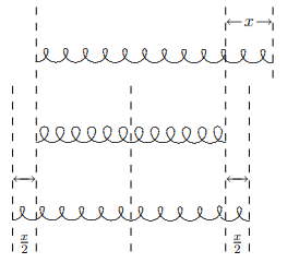
Figure \( 7.1\): Half a spring has twice the spring constant.

According to the discussion above, we can rewrite this as \[\omega^{2}=\frac{K \ell}{\rho_{L}} k^{2}\]

where \(\ell\) is the length of the spring and \(K\) is the spring constant of the spring as a whole.

Note that in longitudinal oscillations in a continuous material in the \(x\) direction, the equilibrium position, \(x\), doesn’t actually describe the \(x\) position of the material. Because the displacement is longitudinal, the actual \(x\) position of the point on the spring with equilibrium position \(x\) is \[x+\psi(x, t),\]

where \(\psi\) is the displacement. You will need this to do problem (7.1).

Fixed Ends

Suppose that we have a massive spring with length \(\ell\) and its ends fixed at \(x = 0\) and \(x = \ell\). Then the displacement, \(\psi(x,t)\) must vanish at the ends, \[\psi(0, t)=0, \quad \psi(\ell, t)=0 .\]

The modes of the system are the same as for any other space translation invariant system. The linear combinations of the complex exponential modes of the infinite system that satisfy (7.6) are \[A_{n}(x)=\sin \frac{n \pi x}{\ell} ,\]

with angular wave number \[k_{n}=\frac{n \pi}{\ell}\]

and frequency (from the dispersion relation, (7.4)) \[\omega_{n}=\sqrt{\frac{K \ell}{\rho_{L}}} k_{n}=\sqrt{\frac{K \ell}{\rho_{L}}} \frac{n \pi}{\ell} .\]

However, because the oscillations are longitudinal, the modes look very different from the transverse modes of the string that we studied in the previous chapter. The position of the point on the string whose equilibrium position is x, in the nth normal mode, has the general form (from (7.5)) \[x+\epsilon \sin \frac{n \pi x}{\ell} \cos \left(\omega_{n} t+\phi\right)\]

where \(\epsilon\) and \(\phi\) are the amplitude and phase of the oscillation.

The lowest 9 modes in (7.10) are animated in program 7-1. Compare these with the modes animated in program 6-1. The mathematics is the same, but the physics is very different because of (7.5). Stare at these two animations until you can visualize the relation between the two. Then you will have understood (7.5).

Free Ends

Now let us look at the situation in which the end of the spring at \(x = 0\) is fixed, but the end at \(x = \ell\) is free. The boundary conditions in this case are analogous to the normal modes of the string with one fixed end. The displacement at \(x = 0\) must vanish because the end is fixed. Also, the derivative of the displacement at \(x = \ell\) must vanish. You can see this by looking at the continuous spring as the limit of discrete masses coupled by springs. As we saw in (5.43), the last real mass must have the same displacement as the first “imaginary” mass, \[\psi(\ell, t)=\psi(\ell+a, t) .\]

Therefore, for the finite system with a free end at \(\ell\), we have the relation \[\frac{\psi(\ell, t)-\psi(\ell+a, t)}{a}=0 \text { for all } a .\]

In the limit that the distance between masses goes to zero, this becomes the condition that the derivative of the displacement, \(\psi\), with respect to \(x\) vanishes at \(x = \ell\), \[\left.\frac{\partial}{\partial x} \psi(x, t)\right|_{x=\ell}=0 .\]

Thus the boundary conditions on the displacement are the same as in (6.11) for the transverse oscillation of a continuous string with \(x = 0\) fixed and \(x = \ell\) free, \[\psi(0, t)=0,\left.\quad \frac{\partial}{\partial x} \psi(x, t)\right|_{x=\ell}=0 .\]

This, in turn, implies that the normal modes are the same as for the transversely oscillating string, (6.15), \[A_{n}(x)=\sin \left(\frac{(2 n+1) \pi x}{2 \ell}\right) \quad \text { for } n=0 \text { to } \infty .\]

However, again because of (7.5), these modes look very different from those of the string. The first nine are animated in program 7-2 (compare with program 6-2).

___________________
¹We will say this much more formally below.