7.2: A Mass on a Light Spring

Let us return to the system that we studied at the very beginning of the book, the harmonic oscillator constructed by putting a mass at the end of a light spring. We are now in a position to understand precisely what “light” means for this system, because we can now allow the spring to have a nonzero linear mass density, \(\rho_{L}\), and find the normal modes of this system. We will then be able to see what happens as \(\rho_{L} \rightarrow 0\).

To be specific, consider a spring with equilibrium length \(\ell\) and spring constant \(K\), fixed at \(x = 0\) and constrained to oscillate only in the \(x\) direction (that is longitudinally). Now attach a mass, \(m\), to the free end (with equilibrium position \(x = \ell\)). The spring, for \(0 < x < \ell\), can be regarded as part of a space translation invariant system. To find the normal modes for this system, we look for linear combination of the modes of the infinite spring (for a given \(\omega\)) that reproduces the physics at \(x = 0\) and \(x = \ell\). The fixed end at \(x = 0\) is easy. This fixes the form of the modes to be proportional to \[\sin k_{n} x\]

with frequency \[\omega_{n}=\sqrt{\frac{K \ell}{\rho_{L}}} k_{n} .\]

As always, \(k_{n}\) and \(\omega_{n}\) are related by the dispersion relation, (7.4). Now to determine the possible values of \(k_{n}\), we require that \(F = ma\) be satisfied for the mass. Suppose, for example, that the amplitude of the oscillation is \(A\) (a length). Then the displacement of the point on the spring with equilibrium position \(x\) is \[\psi(x, t)=A \sin k_{n} x \cos \omega_{n} t,\]

and the displacement of the mass is determined by the displacement of the end of the spring, \[x(t) \equiv \psi(\ell, t)=A \sin k_{n} \ell \cos \omega_{n} t .\]

The acceleration is \[a(t)=\frac{\partial^{2}}{\partial t^{2}} \psi(\ell, t)=-\omega_{n}^{2} A \sin k_{n} \ell \cos \omega_{n} t\]

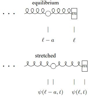
Figure \( 7.2\): The stretching of the last spring is \(\psi(\ell, t)-\psi(\ell-a, t)\)

To find the force on the mass, consider the massive spring as the continuum limit as \(a \rightarrow 0\) of masses connected by massless springs of equilibrium length \(a\), as at the beginning of the chapter. Then the force on the mass at the end is determined by the stretching of the last spring in the series. This, in turn, is the difference between the displacement of the system at \(x = \ell\) and \(x = \ell - a\), as illustrated in Figure \( 7.2\). Thus the force is \[F=-K_{\dot{a}}[\psi(\ell, t)-\psi(\ell-a, t)] .\]

In order to take the limit, \(a \rightarrow 0\), rewrite this as \[F=-K_{a} a \frac{\psi(\ell, t)-\psi(\ell-a, t)}{a} .\]

Now in the continuum limit, \(K_{a}a\) is \(K \ell\), and the last factor goes to a derivative, \(\left.\frac{\partial}{\partial x} \psi(x, t)\right|_{x=\ell}\). The final result for the force is therefore² \[F=-\left.K \ell \frac{\partial}{\partial x} \psi(x, t)\right|_{x=\ell}=-K \ell k_{n} A \cos k_{n} \ell \cos \omega_{n} t .\]

Note that the units work. \(K \ell\) is a force. \(\frac{\partial}{\partial x} \psi\) is dimensionless.

Putting (7.20) and (7.23) into \(F = ma\) and canceling a factor of \(-A \cos \omega_{n} t\) on both sides gives, \[K \ell k_{n} \cos k_{n} \ell=m \omega_{n}^{2} \sin k_{n} \ell .\]

Using the dispersion relation to eliminate \(\omega_{n}^{2}\), we obtain \[k_{n} \ell \tan k_{n} \ell=\frac{\rho_{L} \ell}{m} .\]

We have multiplied both sides of (7.25) by \(\ell\) in order to deal with the dimensionless variables \(k_{n}\ell\) (which is \(2 \pi\) times the number of wavelengths that fit onto the spring) and the dimensionless number \[\epsilon \equiv \frac{\rho_{L} \ell}{m}\]

(which is the ratio of the mass of the spring, \(\rho_{L}\ell\), to the mass, \(m\)). The spring is light if \(\epsilon\) is much smaller than one.

The important point is that (7.25) has only one solution for \(k_{n}\ell\) that goes to zero as \(\epsilon \rightarrow 0\). Because \(\tan k \ell \approx k \ell\) for small \(k \ell\), it is \[k_{0} \ell \approx \sqrt{\epsilon} \text { . }\]

For all the other solutions, the smallness of the left-hand side of (7.25) must come because \(\tan k_{n} \ell\) is very small, \[k_{n} \ell \approx n \pi \quad \text { for } n=1 \text { to } \infty .\]

But (7.28) implies \[x(t) \equiv \psi(\ell, t)=A \sin k_{n} \ell \cos \omega_{n} t \approx 0 \quad \text { for } n=1 \text { to } \infty .\]

In other words, in all the solutions except \(k_{0}\), the mass is hardly moving at all, and the spring is doing almost all the oscillating, looking very much like a system with two fixed ends. Furthermore, the frequencies of all the modes except the \(k_{0}\) mode are large, \[\omega_{n} \approx n \pi \sqrt{\frac{K}{\rho_{L} \ell}} \quad \text { for } n=1 \text { to } \infty ,\]

while the frequency of the \(k_{0}\) mode is \[\omega_{0} \approx \sqrt{\frac{K}{m}} .\]

For small \(\epsilon\) (large mass), the \(k_{0}\) mode is associated primarily with the oscillation of the mass, and has about the frequency we found for the case of the massless spring. The other modes are in an entirely different range of frequencies. They are associated with the oscillations of the spring. This is an important example of the way in which a single system can behave in very different ways in different regimes of frequency.

____________________
²Note that we can use this to give an alternate derivation of the boundary condition for a free end, (7.14).