8.1: Standing and Traveling Waves

What is It That is Moving?

8-1
We have seen that an infinite system with translation invariance has complex solutions of the form \[e^{\pm i k x} e^{\pm i \omega t} ,\]

where \(k\) and \(\omega\) are related by the dispersion relation characteristic of the system. So far, we have considered standing wave solutions in which the space and time dependent factors are separately real, i.e. \[\sin k x \cdot \cos \omega t \propto\left(e^{i k x}-e^{-i k x}\right) \cdot\left(e^{i \omega t}+e^{-i \omega t}\right) .\]

But we can put the same solutions together in a different way, \[\psi(x, t)=\cos (k x-\omega t) \propto\left(e^{i k x} e^{-i \omega t}+e^{-i k x} e^{i \omega t}\right) .\]

This is called a “traveling wave.” The underlying system that supports the wave is not actually traveling. Instead, what is moving is the wave itself. If we follow the point \(x\) for which \(\psi(x,t)\) has some constant value, the point moves in the positive \(x\) direction at a constant velocity, called the “phase velocity,” \[v_{\phi}=\omega(k) / k .\]

In (8.3), for example, \(\psi(x,t)\) is equal to one for \(x = t = 0\), because the argument of the cosine is zero (it is also equal to one for \(x=2 n \pi / k\) for any integer \(n\), but we will focus on just the single point, \(x = 0\)). As \(t\) increases, this point moves in the positive \(x\) direction because the argument of the cosine, \(k x-\omega t\), vanishes for \(x=\omega t / k=v_{\phi} t\). This is illustrated in program 8-1.

We will continue to define all the real modes to be real parts of complex modes proportional to \(e^{-i \omega t}\). Thus (8.3) is \[\cos (k x-\omega t)=\operatorname{Re}\left[e^{i k x} e^{-i \omega t}\right] .\]

In this notation a wave traveling to the left is \[\cos (k x+\omega t)=\operatorname{Re}\left[e^{-i k x} e^{-i \omega t}\right] ,\]

while a standing wave is \[\begin{gathered}
\cos k x \cos \omega t=\frac{1}{2} \operatorname{Re}\left[e^{i k x} e^{-i \omega t}+e^{-i k x} e^{-i \omega t}\right] \\
=\frac{1}{2}[\cos (k x-\omega t)+\cos (k x+\omega t)] .
\end{gathered}\]

A standing wave is a combination of traveling waves going in opposite directions! Likewise, a traveling wave is a combination of standing waves. For example, \[\cos (k x-\omega t)=\cos k x \cos \omega t+\sin k x \sin \omega t .\]

These relations are important because they show that the relation between \(k\) and \(\omega\), the dispersion relation, is just the same for traveling waves as for standing waves! A wave is a wave, whether traveling or standing. Indeed, we can go back and forth using (8.7) and (8.8). The dispersion relation that relates \(k\) and \(\omega\) is a property of the system in which the waves exist, not of the particular wave.

The other side of this coin is that traveling waves exist for systems with any dispersion relation. Knowing the phase velocity, (8.4), for all \(k\) is equivalent to knowing the dispersion relation, because you must know \(\omega(k)\). In particular, it is only for simple, continuous systems like the stretched string (see (6.5)) that \(\omega(k)\) is proportional to \(k\) and the phase velocity is a constant, independent of \(k\).

Boundary Conditions

8-2
Traveling waves can be produced in finite systems by forced oscillation with an appropriate phase for the oscillations at the two ends. A simple example involves a stretched string with tension \(T\) and linear mass density \(\rho\). Given boundary conditions on the system so that \[\psi(0, t)=A \cos \omega t, \quad \psi(L, t)=A \sin \omega t ,\]

where \(L\) is the length of the string, the angular frequency \(\omega\) is chosen so that \[k=\frac{5 \pi}{2 L}=\omega \sqrt{\frac{\rho}{T}}=\frac{\omega}{v_{\phi}} .\]

As usual in a forced oscillation problem, we are interested in the steady state solution in which the system moves with the angular frequency, \(\omega\), of the forcing terms. We can solve this problem easily by breaking it up into two problems.

First consider the boundary condition: \[\psi_{1}(0, t)=0, \quad \psi_{1}(L, t)=A \sin \omega t .\]

This is easily solved by the methods of chapter 5. From the condition at \(x = 0\), we know that the solution for \(\psi_{1}(x, t)\) is proportional to \(\sin k x\). Then the boundary condition at \(x = L\) gives the standing wave solution: \[\psi_{1}(x, t)=A \sin k x \sin \omega t .\]

Next consider the boundary condition \[\psi_{2}(0, t)=A \cos \omega t, \quad \psi_{2}(L, t)=0 .\]

Analogous arguments (starting at \(x = L\)) show that the solution is the standing wave \[\psi_{2}(x, t)=A \cos k x \cos \omega t .\]

Now we can obtain the solution for the boundary condition (8.9) simply by adding these: \[\begin{gathered}
\psi(x, t)=\psi_{1}(x, t)+\psi_{2}(x, t) \\
=A \cos k x \cos \omega t+A \sin k x \sin \omega t=A \cos (k x-\omega t) ,
\end{gathered}\]

which is a wave traveling from \(x = 0\) to \(x = L\). The crucial point is that the two standing waves out of which the traveling wave is built are \(90^{\circ}\) out of phase with one another both in time and in space. They get large at different points in space and also at different times and the interplay between the two produces the traveling wave. This is illustrated in \(Figures \text { } 8.1 \text {-} 8.4\) for \(\omega t = 0\), \(\pi / 4\), \(\pi / 2\) and \(3 \pi / 4\). In each of these figures, the top curve is the traveling wave. The middle curve is (8.14). The lower curve is (8.12).

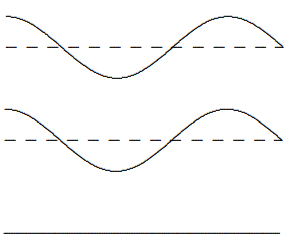
Figure \( 8.1\): \(t = 0\).

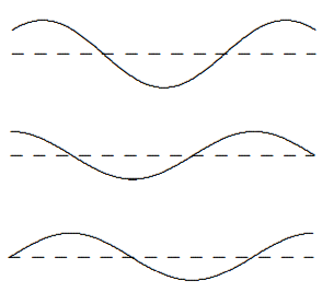
Figure \( 8.2\): \(t = \pi / 4\).

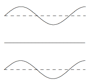
Figure \( 8.3\): \(t = \pi / 2\).

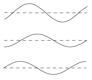
Figure \( 8.4\): \(t = 3 \pi / 4\).

This system is animated in program 8-2. This animation is important. It is worth staring at it for a while to get a better feeling for how (8.15) works than you can from the still pictures in \(Figures \text { } 8.1 \text{-} 8.4\). If you concentrate on a particular point on the string, you will see that the traveling wave gets large either when one of the standing waves is a maximum with the other near zero, or (depending on where you looking) when both standing waves are positive.