8.4: Transmission Lines

We have seen that a translation invariant system of inductors and capacitors can carry waves. Let us ask what happens when we take the continuum limit of such a system. This will give an interesting insight into electromagnetic waves. The dispersion relation for the system of Figure \( 5.23\) is given by (5.75), \[\omega^{2}=\frac{4}{L_{a} C_{a}} \sin ^{2} \frac{k a}{2} .\]

where \(L_{a}\) and \(C_{a}\) are the inductance and capacitance of the inductors and capacitors for the system with separation \(a\) between neighboring parts. To take the continuum limit, we must replace the inductance and capacitance, \(L_{a}\) and \(C_{a}\), by quantities that we expect to have finite limits as \(a \rightarrow 0\). We expect from the analogy, (5.69), between \(LC\) circuits and systems of springs and masses, and the discussion at the beginning of chapter 7 about the continuum limit of the system of masses and springs that the relevant quantities will be: \[\begin{aligned}
&\rho_{L} \rightarrow \frac{L_{a}}{a} \quad \text { inductance per unit length } \\
&K_{a} a \rightarrow \frac{a}{C_{a}} \quad \text { capacitance per unit length }
\end{aligned}\]

These two quantities can be computed directly from the inductance and capacitance of a finite length, \(\ell\), of the system that contains many individual units. The inductances are connected in series so the individual inductances add to give the total inductance. Thus if the length \(\ell\) is \(na\) so that if the finite system contains \(n\) inductors, the total inductance is \(L = n L_{a}\). Then \[\frac{L}{\ell}=\frac{L_{a}}{a}\]

The capacitances work the same way because they are connected in parallel, and parallel capacitances add. Thus \[\frac{C}{\ell}=\frac{C_{a}}{a} .\]

Therefore, in taking the limit as \(a \rightarrow 0\) of (8.49), we can write \[L_{a}=a \frac{L}{\ell}, \quad C_{a}=a \frac{C}{\ell} .\]

This gives the following dispersion relation: \[\omega^{2}=\frac{\ell^{2}}{L C} \frac{4 \sin ^{2} \frac{k a}{2}}{a^{2}} \rightarrow \frac{\ell^{2}}{L C} k^{2} .\]

A continuous system like this with fixed inductance and capacitance per unit length is called a transmission line. We will call (8.54) the dispersion relation for a resistanceless transmission line. A transmission line can be used to send electrical waves, just as a continuous string transmits mechanical waves. In the continuous system, the displacement variable, the displaced charge, becomes a function of position along the transmission line. If the transmission line is stretched in the \(z\) direction, we can describe the charges on the transmission line by a function \(Q(z,t)\) that is the charge that has been displaced through the point \(z\) on the transmission line at time \(t\). The time derivative of \(Q(z,t)\) is the current at the point \(z\) and time \(t\): \[I(z, t)=\frac{\partial Q(z, t)}{\partial t} .\]

Parallel Plate Transmission Line

It is worth working out a particular example of a transmission line. The example we will use is of two long parallel conducting strips. Imagine an infinite system in which the strips are stretched parallel to one another in planes of constant \(y\), going to infinity in the \(z\) direction. Suppose that the strips are sufficiently thin that we can neglect their thickness. Suppose further that the width of strips, \(w\), is much larger than the separation, \(s\). A cross section of this transmission line in the \(x - y\) plane is shown in Figure \( 8.9\). In the figure, the \(z\) direction is out of the plane of the paper, toward you. We will keep track of the motion of the charges in the upper conductor and assume that the lower conductor is grounded (with voltage fixed at \(V = 0\)).

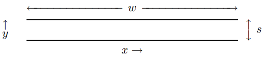
Figure \( 8.9\): Cross section of a transmission line in the \(x - y\) plane.

We will find the dispersion relation of the transmission line by computing the capacitance and inductance of a part of the line of length \(\ell\). It will be useful to do this using energy considerations. Suppose that there is a charge, \(Q\), uniformly spread over the upper plate of the capacitor, and a current, \(I\), flowing evenly out of the \(x - y\) plane in the \(z\) direction along the upper conductor (and back into the plane along the lower conductor). The energy stored in the length, \(\ell\), of the transmission line is then \[\frac{1}{2 C} Q^{2}+\frac{1}{2} L I^{2} ,\]

where \(C\) and \(L\) are the capacitance and inductance.⁴

The energy is actually stored in the electric and magnetic fields produced by the charge and current. In this configuration, the electric and magnetic fields are almost entirely between the two plates of the piece of the transmission line. If \(Q\) and \(I\) are positive, the electric and magnetic fields are as shown in Figure \( 8.10\) and Figure \( 8.11\). In Figure \( 8.10\), the dotted line is a cross section of a box-shaped region that can be used to compute the electric field, using Gauss’s law. In Figure \( 8.11\), the dotted path can be used to compute the magnetic field, using Ampere’s law. The electric and magnetic fields are approximately constant between the strips, but quickly fall off to near zero outside.

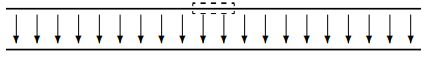
Figure \( 8.10\): The electric field due to the charge on the transmission line.

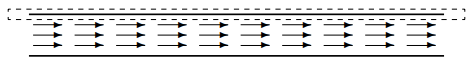
Figure \( 8.11\): The magnetic field due to the current on the transmission line.

The charge density on the upper plate is approximately uniform and given by the total charge divided by the area, \(w \ell\), \[\sigma \approx \frac{Q}{w \ell} .\]

Then we can apply Gauss’s law to a small box-shaped region, a cross section of which is shown in Figure \( 8.10\) and conclude that the electric field inside is given by \[E_{y} \approx-\frac{Q}{\epsilon_{0} w \ell}\]

The density of energy stored in the electric field between the plates is therefore \[u_{E}=\frac{\epsilon_{0}}{2} E^{2} \approx \frac{Q^{2}}{2 \epsilon_{0} w^{2} \ell^{2}} .\]

The total energy stored in the electric field is then obtained by multiplying \(u_{E}\) by the volume between the plates, yielding \[\frac{1}{2} \frac{s}{\epsilon_{0} w \ell} Q^{2}\]

thus (comparing with (8.56)) \[C=\frac{\epsilon_{0} w \ell}{s} .\]

We can calculate the inductance in a similar way. Ampere’s law, applied to a path enclosing the upper conductor (as shown in figure 8.11) gives \[B_{x} \approx \frac{\mu_{0} I}{w} .\]

The density of energy stored in the magnetic field between the plates is therefore \[u_{B}=\frac{1}{2 \mu_{0}} B^{2} \approx \frac{\mu_{0} I^{2}}{2 w^{2}} .\]

The total energy stored in the magnetic field is then obtained by multiplying \(u_{B}\) by the volume between the plates, yielding \[\frac{1}{2} \frac{\mu_{0} s \ell}{w} I^{2}\]

thus (comparing with (8.56)) \[L=\frac{\mu_{0} s \ell}{w} .\]

We can now put (8.61) and (8.65) into (8.54) to get the dispersion relation for this transmission line: \[\omega^{2}=\frac{1}{\mu_{0} \epsilon_{0}} k^{2}=c^{2} k^{2} ,\]

where \(c\) is the speed of light!

Waves in the Transmission Line

The dispersion relation, (8.66), looks suspiciously like the dispersion relation for electromagnetic waves. In fact, the electric and magnetic fields between the strips of the transmission line have exactly the form of an electromagnetic wave. To see this explicitly, let us look at a traveling wave on the transmission line, and consider the charge, \(Q(z,t)\), displaced through \(z\), with the irreducible complex exponential \(z\) and \(t\) dependence, \[Q(z, t)=q e^{i(k z-\omega t)} .\]

This wave is traveling in the positive \(z\) direction, out toward you in the diagram of Figure \( 8.9\).

At any fixed time, \(t\) and position, \(z\), the electric and magnetic fields inside the transmission line look as shown in Figure \( 8.10\) and Figure \( 8.11\) (or both may point in the opposite direction). We can find the magnetic field just as we did above, because the current at any point along the line is given by (8.55), so \[B_{x}(z, t) \approx \frac{\mu_{0} I(z, t)}{w}=\frac{\mu_{0}}{w} \frac{\partial}{\partial t} Q(z, t)=-i \frac{\mu_{0} \omega q}{w} e^{i(k z-\omega t)} .\]

To find the electric field as a function of \(z\) and \(t\), we need the density of charge along the line. Once we have that, we can find the electric field using Gauss’s law, as above. A nonzero charge density results if the amount of charge displaced changes as a function of \(z\). It is easiest to find the charge density by returning to the discrete system discussed in chapter 5, and to (5.72). In the language in which we label the parts of the system by their positions, the charge, \(q_{j}\), in the discrete system becomes \(q(z,t)\) where \(z = j a\). As \(a \rightarrow 0\), this corresponds to a linear charge density along the transmission line of \[\rho(z, t)=\frac{q(z, t)}{a} .\]

In this language, (5.72) becomes \[q(z, t)=Q(z, t)-Q(z+a, t) ,\]

where \(Q(z,t)\) is the charge displaced through the inductor a position \(z\) at time \(t\). Combining (8.69) and (8.70) gives \[\rho(z, l)=\frac{Q(z, t)-Q(z+a, t)}{a} .\]

Taking the limit as \(a \rightarrow 0\) gives \[\rho(z, t)=-\frac{\partial}{\partial z} Q(z, t)=-i k q e^{i(k z-\omega t)} .\]

This linear charge density is spread out over the width of the upper strip in the transmission line, giving a surface charge density of \[\sigma(z, t)=\frac{\rho(z, t)}{w}=-i \frac{k q}{w} e^{i(k z-\omega t)} .\]

Now the electric field from Gauss’s law is \[E_{y}=-\frac{\sigma(z, t)}{\epsilon_{0}}=i \frac{k q}{\epsilon_{0} w} e^{i(k z-\omega t)} .\]

Comparing (8.68) with (8.74), you can see that (8.45) is satisfied, so that this pair of electric and magnetic fields form a part of a traveling electromagnetic plane wave.

What is happening here is that the role of the charges and currents in the strips of the transmission line is to confine the electromagnetic waves. Without the conductors it would impossible to produce a piece of a plane wave, as we will see in much more detail in chapter 13.

Meanwhile, note that the mode with \(\omega = 0\) and \(k = 0\) must be treated with care, as with the \(\omega = k = 0\) mode of the beaded string discussed in chapter 5. The mode in which the displaced charge is proportional to \(z\) (see (5.41)) describes a situation in which the entire infinite transmission line is charged. This is not very interesting in the finite case. However, the mode that is independent of \(z\), but increasing with time, proportional to \(t\) is important. This describes the situation in which a constant current is flowing through the conductors. Inside the transmission line, in this case, is a constant magnetic field.

____________________
⁴See Haliday and Resnick, part 2.