8.3: Light

Light waves, like the sound waves that we discussed in the previous chapter, are inherently three-dimensional things. However, as with sound, we can say a lot about light that is more or less independent of the three-dimensional details.

Plane Waves

There is a simple way of concentrating on only one dimension. That is to look for solutions in which the other two dimensions do not enter at all. Consider Maxwell’s equations in free space, in terms of the vector fields, \(\vec{E}\) and \(\vec{B}\) describing the electric and magnetic fields. \[\begin{aligned}
&\frac{\partial E_{y}}{\partial x}-\frac{\partial E_{x}}{\partial y}=-\frac{\partial B_{z}}{\partial t} \\
&\frac{\partial E_{z}}{\partial y}-\frac{\partial E_{y}}{\partial z}=-\frac{\partial B_{x}}{\partial t} \\
&\frac{\partial E_{x}}{\partial z}-\frac{\partial E_{z}}{\partial x}=-\frac{\partial B_{y}}{\partial t}
\end{aligned}\]

\[\begin{aligned}
&\frac{\partial B_{y}}{\partial x}-\frac{\partial B_{x}}{\partial y}=\mu_{0} \epsilon_{0} \frac{\partial E_{z}}{\partial t} \\
&\frac{\partial B_{z}}{\partial y}-\frac{\partial B_{y}}{\partial z}=\mu_{0} \epsilon_{0} \frac{\partial E_{x}}{\partial t} \\
&\frac{\partial B_{x}}{\partial z}-\frac{\partial B_{z}}{\partial x}=\mu_{0} \epsilon_{0} \frac{\partial E_{y}}{\partial t}
\end{aligned}\]

\[\begin{aligned}
&\frac{\partial E_{x}}{\partial x}+\frac{\partial E_{y}}{\partial y}+\frac{\partial E_{z}}{\partial z}=0 \\
&\frac{\partial B_{x}}{\partial x}+\frac{\partial B_{y}}{\partial y}+\frac{\partial B_{z}}{\partial z}=0
\end{aligned}\]

where \(\epsilon_{0}\) and \(\mu_{0}\) are two constants called the permittivity and permeability of empty space.³ Let us look for solutions to these partial differential equations that involve only functions of \(z\) and \(t\). In this case, things simplify to: \[0=-\frac{\partial B_{z}}{\partial t}, \quad-\frac{\partial E_{y}}{\partial z}=-\frac{\partial B_{x}}{\partial t}, \quad \frac{\partial E_{x}}{\partial z}=-\frac{\partial B_{y}}{\partial t} ,\]

\[0=\mu_{0} \epsilon_{0} \frac{\partial E_{z}}{\partial t}, \quad-\frac{\partial B_{y}}{\partial z}=\mu_{0} \epsilon_{0} \frac{\partial E_{x}}{\partial t}, \quad \frac{\partial B_{x}}{\partial z}=\mu_{0} \epsilon_{0} \frac{\partial E_{y}}{\partial t} ,\]

\[\frac{\partial E_{z}}{\partial z}=0, \quad \frac{\partial B_{z}}{\partial z}=0 .\]

These equations imply that \(E_{z}\) and \(B_{z}\) are independent of \(z\) and \(t\). Since we have already assumed that they depend only on \(z\) and \(t\), this means that they are constants. We will ignore them because we are interested in the solutions with nontrivial \(z\) and \(t\) dependence. That leaves the \(x\) and \(y\) components, satisfying (8.38) and (8.39).

Then, because (8.38) and (8.39) are invariant under translations in \(z\) and \(t\), we expect complex exponential solutions, in which all components are proportional to \[e^{i(\pm k z-\omega t)},\]

\[E_{x}(z, t)=\varepsilon_{x}^{\pm} e^{i(\pm k z-\omega t)}, \quad E_{y}(z, t)=\varepsilon_{y}^{\pm} e^{i(\pm k z-\omega t)} ,\]

\[B_{x}(z, t)=\beta_{x}^{\pm} e^{i(\pm k z-\omega t)}, \quad B_{y}(z, t)=\beta_{y}^{\pm} e^{i(\pm k z-\omega t)} ,\]

Direct substitution of (8.42) and (8.43) into (8.38) and (8.39) gives \[\mp k \varepsilon_{y}^{\pm}=\omega \beta_{x}^{\pm}, \quad \pm k \varepsilon_{x}^{\pm}=\omega \beta_{y}^{\pm},\]

\[\mp k \beta_{y}^{\pm}=-\mu_{0} \epsilon_{0} \omega \varepsilon_{x}^{\pm}, \quad \pm k \beta_{x}^{\pm}=-\mu_{0} \epsilon_{0} \omega \varepsilon_{y}^{\pm} .\]

As usual, we have written the wave with the irreducible time dependence, \(e^{-i \omega t}\). To get the real electric and magnetic fields, we take the real part of (8.42) and (8.43). This works because Maxwell’s equations are linear in the electric and magnetic fields. The amplitudes, \(\varepsilon_{x}^{\pm}\), etc, can be complex.

From (8.44) and (8.45), you see that \(\varepsilon_{y}^{\pm}\) is related to \(\beta_{x}^{\pm}\) and \(\varepsilon_{x}^{\pm}\) is related to \(\beta_{y}^{\pm}\). For each relation, there are two homogeneous simultaneous linear equations in the two unknowns. They are consistent only if the ratio of the coefficients is the same, which implies a relation between \(k\) and \(\omega\), \[k^{2}=\mu_{0} \epsilon_{0} \omega^{2} .\]

This is a dispersion relation, \[\omega^{2}=c^{2} k^{2}=\frac{1}{\mu_{0} \epsilon_{0}} k^{2} .\]

The phase velocity, \(c\), is the speed of light in vacuum (we will have more to say about this in chapters 10 and 11!).

Once (8.47) is satisfied, we can solve for the \(\beta^{\pm}\) in terms of the \(\varepsilon^{\pm}\): \[\beta_{y}^{\pm}=\pm \frac{1}{c} \varepsilon_{x}^{\pm}, \quad \beta_{x}^{\pm}=\mp \frac{1}{c} \varepsilon_{y}^{\pm} .\]

These solutions to Maxwell’s equations in free space are electromagnetic waves, or light waves. These simple solutions, depending only on \(z\) and \(t\) are an example of plane wave solutions. The name is appropriate because the electric and magnetic fields in the wave have the same value everywhere on each plane of constant \(z\), for any fixed time, \(t\). These planes propagate in the \(\pm z\) direction at the phase velocity, \(c\).

In general, electromagnetic waves can propagate in any direction in three-dimensional space. However, the electric and magnetic fields that make up the wave are always perpendicular to the direction in which the wave is traveling and perpendicular to each other.

The treatment of plane wave electromagnetic waves traveling in the \(z\) direction is analogous to our treatment of sound in chapter 7. There, also, the wave depended only on \(z\). However, the electromagnetic waves are a little more complicated because the wave phenomenon depends on both the electric and magnetic fields. The reason that we have postponed until now the discussion of electromagnetic waves, even though they are one of the most important examples of wave phenomena, is that the relations, (8.48), between the electric and magnetic fields depend on the direction in which the wave is traveling (the \(\pm\) sign!). It is much easier to write down the solutions for the traveling waves than for the standing waves. Even for the simple traveling plane waves we have described that depend only on \(z\) and \(t\), this relation between \(\vec{E}\) and \(\vec{B}\) and the direction of the wave depends on the three-dimensional properties of Maxwell’s equations. We will discuss these issues in much more detail in chapters 11 and 12.

Interferometers

One of the wonderful features of light waves is that it is relatively easy to split them up and reassemble them. This feature is used in many optical devices, one of the simplest of

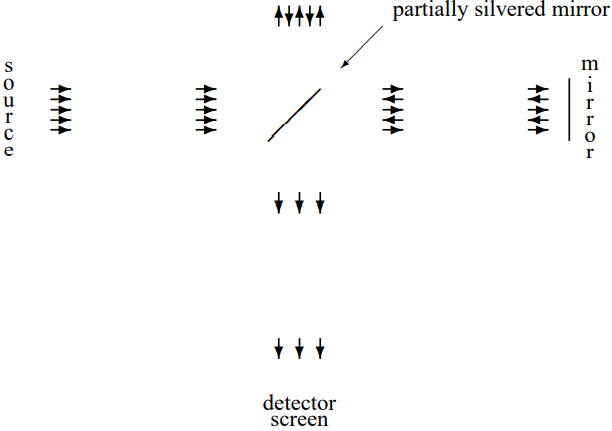
Figure \( 8.8\): A schematic diagram of a Michelson interferometer.

which is an “interferometer,” one version of which (the Michelson interferometer) is shown in schematic form in Figure \( 8.8\). A source produces a plane wave (as we will discuss in chapter 13, it cannot be quite a plane wave, but never mind that for now). The partially silvered mirror serves as a “beam splitter” by allowing some of the light to pass through, while reflecting the rest. Then the mirrors at the top and the right reflect the beams back. Then the partially silvered mirror serves as a “beam reassembler,” combining the beams from the top and the right into a single beam that travels on to the detector screen where the beam intensity (proportional to the square of the electric field) is measured. The important thing is that the light wave reaching the detector screen is the sum of two components that are coherent and yet have traveled different paths. What “coherent” means in this context is not only that the frequency is the same, but that the phase of the waves is correlated. In this case, that happens simply because the two components reaching the screen arise from the same incoming plane wave.

Now the intensity of the light reaching the screen depends on the relative length of the two paths. Different path lengths will produce different phases. If the two components are in phase, the amplitudes will add and the screen will be bright. This is called “constructive interference”. If the two components are \(180^{\circ}\) out of phase, the amplitudes will subtract and the screen will be dark. There will be what is called “destructive interference.”

This sounds rather trivial, and indeed it is (at least for classical electromagnetic waves), but it is also extremely useful, because it provides a very sensitive measure of changes of the length of the paths. In particular, if one of the mirrors is moved a distance \(d\) (it might be part of an experimental setup designed to detect small motions, for example), the relative phase of the two components reaching the screen changes by \(2kd\) where \(k\) is the angular wave number of the plane wave, because the path length of the reflected wave has changed by \(2d\). Thus each time \(d\) changes by a quarter of the wavelength of the light, the screen goes from bright to dark, or vice versa.

This is a very useful way of measuring small distance changes. In practice, the incoming beam is not exactly a plane wave (that, as we will see in detail later, would require an infinite experiment!), so the intensity of the light is not uniform over the screen. Instead there are light areas and dark areas known as “fringes.” As the mirror is moved, the fringes move, and one can count the fringes that go past a given spot to keep track of the number of changes from bright to dark.

Quantum Interference

There is another wave of thinking about the interferometer that makes it seem much less trivial. As we will discuss several times in this book, and you will learn more about when you study quantum mechanics, light is not only a wave. It is also made up of individual particles of light called photons. You don’t notice this unless you turn the intensity of the light wave way down. But in fact, you can turn the intensity down so much that you can detect individual photons hitting the screen. Now it is not so clear what is happening. An individual photon cannot split into two parts at the beam splitter and beam reassembler. As we will see later, the energy of the photon is determined by the frequency of the light. It cannot be divided. You might think, therefore, that the individual photon would have to go one way or the other. But then how can one get an interference between the two paths? There is no answer to this question that makes “sense” in the classical physics of particles. Nevertheless, when the experiment is done, the number of photons reaching the screen depends on the difference in lengths between the two paths in just the way you expect from the wave description! The probability that a photon will hit a given spot on the screen is proportional to the intensity of the corresponding classical wave. If the path lengths produce destructive interference, no photons get through. Not only that, but similar experiments can be done with other particles, such as neutrons! Maybe interference is not so trivial after all.

___________________________
³See, for example, Purcell, chapter 9.