8.6: High and Low Frequency Cut-Offs

More on Coupled Pendulums

8-6
In the previous section, we saw how the angular wave number, \(k\), can become complex in a system with friction. There is another important way in which \(k\) can become complex. Consider the dispersion relation for the system of coupled pendulums, (5.35), which we can rewrite as follows: \[\omega^{2}=\omega_{\ell}^{2}+\omega_{c}^{2} \sin ^{2} \frac{k a}{2} .\]

Here \(a\) is interblock distance, \(\omega_{\ell}\) is the frequency of a single uncoupled pendulum, and \(\omega_{c}^{2}\) is a frequency associated with the coupling between neighboring blocks. \[\omega_{c}^{2}=\frac{4 K}{m}\]

where \(m\) is the mass of a block and \(K\) is the spring constant of the coupling springs.

Traveling waves in a system with a dispersion relation like (8.92) are animated in program 8-6. To make the physics easier to see, this system is a beaded string with transverse oscillations. However, to produce the \(\omega_{\ell}^{2}\) term in (8.92), we have also attached each bead by a spring to an equilibrium position along the dotted line. In this case, the coupling between beads comes from the string, so the analog of (8.93) is \[\omega_{c}^{2}=\frac{4 T}{m a} .\]

The parameters in the system are chosen so that in terms of a reference frequency, \(\omega_{0}\), \[\omega_{\ell}^{2}=25 \omega_{0}^{2}, \quad \omega_{c}^{2}=24 \omega_{0}^{2}\]

The properties of waves in this system differ dramatically as a function of \(\omega\). One way to see this is to go backwards and note that for real \(k\), because \(\sin ^{2} \frac{k a}{2}\) must be between 0 and 1, \(\omega\) is constrained, \[\omega_{\ell} \leq \omega \leq \sqrt{\omega_{\ell}^{2}+\omega_{c}^{2}} \equiv \omega_{h}\]

For \(k\) in this “allowed” region, \[\sin ^{2} \frac{k a}{2}=\frac{\omega^{2}-\omega_{\ell}^{2}}{\omega_{c}^{2}}\]

is between 0 and 1, as is \[\cos ^{2} \frac{k a}{2}=\frac{\omega_{h}^{2}-\omega^{2}}{\omega_{c}^{2}} .\]

The two frequencies, \(\omega_{\ell}\) and \(\omega_{h}\), are called low and high frequency cut-offs. The system of coupled pendulums supports traveling waves only for frequency \(\omega\) between the high and low frequency cut-offs. It is only in this region that the dispersion relation can be satisfied for real \(\omega\) and \(k\). For \(\omega<\omega_{\ell}\) or |(\omega > \omega_{h}\), the system oscillates, but there is nothing quite like a traveling wave. You can see this in program 8-6 by changing the frequency up and down with the arrow keys.

For any \(\omega\), we can always solve the dispersion relation. However, in some regions of frequency, the result will be complex, as in (8.85). We expect \(k_{i} = 0\) in the allowed region (8.96). The solution of (8.92) for \(k_{r}\) and \(k_{i}\) as functions of \(\omega\) are shown in the graphs in Figure \( 8.12\). Here, \(k_{r}\) and \(k_{i}\) are plotted against \(\omega\) for the dispersion relation, (8.92), with \(\omega_{\ell}=5 \omega_{0}\) and \(\omega_{h}=7 \omega_{0} . k_{i}\). \(k_{i}\) is the dotted line. Note the very rapid dependence of ki near the high and low frequency cut-offs.

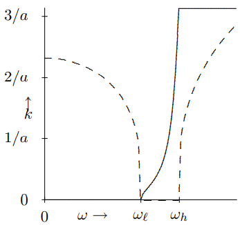
Figure \( 8.12\): \(k_{r}a\) and \(k_{i}a\) versus \(\omega\).

As \(\omega\) decreases, in the allowed region, (8.96), \(\sin \frac{k a}{2}\) decreases. At the low frequency cut-off, \(\omega=\omega_{\ell}\), \(\sin \frac{k a}{2}\) and therefore \(k\) goes to zero. This means that as the frequency decreases, the wavelength of the traveling waves gets longer and longer, until at the cut-off frequency, it becomes infinite. At the low frequency cut-off, every pendulum in the infinite chain is oscillating in phase. The springs that couple them are then irrelevant because they always maintain their equilibrium lengths. This is possible precisely because \(\omega_{\ell}\) is the oscillation frequency of the uncoupled pendulum, so that no coupling is required for an individual pendulum to swing at frequency \(\omega_{\ell}\).

If \(\omega\) is below the low frequency cut-off, \(\omega_{\ell}\), \(\sin \frac{k a}{2}\) must become negative to satisfy the dispersion relation, (8.92). Therefore \(\sin \frac{k a}{2}\) must be a pure imaginary number \[k-\pm i k_{i} .\]

The general solution for the wave is then \[\psi(x, t)=A e^{-k_{i} x} e^{-i \omega t}+B e^{k_{i} x} e^{-i \omega t}\]

In a finite system of coupled pendulums, both terms may be present. In a semi-infinite system that is driven at \(x = 0\) and extends to \(x \rightarrow \infty\), the constant \(B\) must vanish to avoid exponential growth of the wave at infinity. Thus the wave falls off exponentially at large \(x\). Furthermore, the solution is a product of a real function of \(x\) and a complex exponential function of \(t\). This is a standing wave. There is no traveling wave. You can see this in program 8-6 at low frequencies.

The physics of this oscillation below the low frequency cut-off is particularly clear in the extreme limit, \(\omega \rightarrow 0\). At zero frequency, there is no motion. The analog of a forced oscillation problem is just to displace one pendulum from equilibrium and look to see what happens to the rest. Clearly, what happens is that the displacement of the first pendulum causes a force on the next one because of the coupling spring that pulls it away from equilibrium, but not as far as the first. Its displacement is smaller than that of the first by some factor \(\epsilon=e^{-k_{i} a}\). Then the second pendulum pulls the third, but again the displacement is smaller by the same factor. And so on! In an infinite system, this gives rise to the exponentially falling displacement in (8.100) for \(B = 0\). As the frequency is increased, the effect of inertia (more precisely, the \(ma\) term in \(F = ma\)) increases the displacement of second (and each subsequent) block, until above the low frequency cut-off, the effect of inertia is large enough to compete on an equal footing with the effect of the restoring force, and a real traveling wave can be produced.

The low frequency cut-off is not peculiar to the discrete system. It occurs any time there is a restoring force for \(k = 0\) in the infinite system. Later, in chapter 11, we will see that a similar phenomena can occur in two- and three-dimensional systems even when there is no restoring force at \(k = 0\).

The high frequency cut-off, on the other hand, depends on the finite separation between blocks. As \(\omega\) increases, in the allowed region, (8.96), \(\sin \frac{k a}{2}\) increases, \(k\) increases, and therefore \(\cos \frac{k a}{2}\) decreases. At the high frequency cut-off, \(\omega=\omega_{h}), \(\sin \frac{k a}{2}=1\) and \(\cos \frac{k a}{2}= 0\). But \[\sin \frac{k a}{2}=1 \Rightarrow k=\frac{\pi}{a} \]

which, in turn means \[e^{i k a}=e^{-i k a}=-1 .\]

Thus the displacement of the blocks simply alternates, because \[\psi_{j}=\psi(j a, t) \propto e^{i j \pi}=(-1)^{j} .\]

This is as wavy as the discrete system can get. In a discrete system with interblock separation, a, the maximum possible real part of \(k\) is \(\frac{\pi}{a}\) (because \(k\) can be redefined by a multiple of \(\frac{2 \pi}{a}\) without changing the displacements of any of the blocks – see (5.28)). This bound is the origin of the high frequency cut-off.

You can see this in program 8-6. The frequency starts out at \(6 \omega_{0}\). At this point, \(k_{r}a\) is quite small (and \(k_{i} = 0\)) and the wave looks smooth. As the frequency is increased toward \(\omega_{h}\), the wave gets more and more jagged looking, until at \(\omega = \omega_{h}\), neighboring beads are moving in opposite directions.

For \(\omega > \omega_{h}\), \(\sin \frac{k a}{2}\) is greater than 1, and \(\cos \frac{k a}{2}\) is negative. This implies that \(k\) has the form \[k=\frac{\pi}{a} \pm i k_{i} .\]

Then the general solution for the displacement is \[\psi(x, t)=A e^{-k_{i} x} e^{i \pi x / a} e^{-i \omega t}+B e^{k_{i} x} e^{i \pi x / a} e^{-i \omega t} .\]

As in (8.100), there is an exponentially falling term and an exponentially growing one. Here however, there is also a phase factor, \(e^{i \pi x / a}\), that looks as if it might lead to a traveling wave. But in fact, this is not really a phase. It simply produces the alternation of the displacement from one block to the next. We see this if we look only at the displacements of the blocks (as in (8.103), \[\psi_{j}=\psi(j a, t)=A(-1)^{j} e^{-k_{i} x} e^{-i \omega t}+B(-1)^{j} e^{k_{i} x} e^{-i \omega t} .\]

As for (8.100), in a semi-infinite system that extends to \(x \rightarrow \infty\), we must have \(B = 0\), and there is no travelling wave.

One of the striking things about program 8-6 is the very rapid switch from a traveling wave solution in the allowed region to a standing wave solution with a rapid exponential decay of the amplitude in the high and low frequencies regions. You see this also in Figure \( 8.12\) in the rapid change of \(k_{i}\) near the cut-offs. The reason for this is that \(k\) has a square-root dependence on the frequency near the cut-offs.

In the infinite system, the solution outside the allowed region is a pure standing wave. In the absence of damping, the work done by the force that produces the wave averages to zero over time. In a finite system, however, it is possible to transfer energy from one end of a system to the other, even if you are below the low frequency cut-off or above the high-frequency cutoff. The reason is that in a finite system, both the \(A\) and \(B\) terms in (8.100) (or (8.106)) can be nonzero. If \(A\) and \(B\) are both real (or relatively real — that is if they have the same phase), then there is no energy transfer. The solution is the product of a real function of \(x\) (or \(j\)) and an oscillating exponential function of \(t\). Thus it looks like a standing wave. However if \(A\) and \(B\) have different phases, then the oscillation looks something like a traveling wave and energy can be transferred. This process becomes exponentially less efficient as the length of the system increases. We will discuss this in more detail in chapter 11.