10.1: Signals in Forced Oscillation

Pulse on a String

10-1
We begin with the following illustrative problem: the transverse oscillations of a semiinfinite string stretched from \(x = 0\) to \(\infty\), driven at \(x = 0\) with some arbitrary transverse signal \(f(t)\), and with a boundary condition at infinity that there are no incoming traveling waves. This simple system is shown in Figure \( 10.1\).

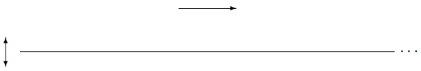
Figure \( 10.1\): A semiinfinite string.

There is a slick way to get the answer to this problem that works only for a system with the simple dispersion relation, \[\omega^{2}=v^{2} k^{2} .\]

The trick is to note that the dispersion relation, (10.1), implies that the system satisfies the wave equation, (6.4), or \[\frac{\partial^{2}}{\partial t^{2}} \psi(x, t)=v^{2} \frac{\partial^{2}}{\partial x^{2}} \psi(x, t) .\]

It is a mathematical fact (we will discuss the physics of it below) that the general solution to the one-dimensional wave equation, (10.2), is a sum of right-moving and left-moving waves with arbitrary shapes, \[\psi(x, t)=g(x-v t)+h(x+v t) ,\]

where \(g\) and \(h\) are arbitrary functions. You can check, using the chain rule, that (10.3) satisfies (10.2), \[\begin{gathered}
\frac{\partial^{2}}{\partial t^{2}}(g(x-v t)+h(x+v t))=v^{2} \frac{\partial^{2}}{\partial x^{2}}(g(x-v t)+h(x+v t)) \\
=v^{2}\left(g^{\prime \prime}(x-v t)+h^{\prime \prime}(x+v t)\right) .
\end{gathered}\]

Given this mathematical fact, we can find the functions \(g\) and \(h\) that solve our particular problem by imposing boundary conditions. The boundary condition at infinity implies \[h = 0\]

because the \(h\) function describes a wave moving in the \(-x\) direction. The boundary condition at \(x = 0\) implies \[g(-v t)=f(t) ,\]

which gives \[\psi(x, t)=f(t-x / v)\]

This describes the signal, \(f(t)\), propagating down the string at the phase velocity \(v\) with no change in shape.

For the simple function \[f(t)=\left\{\begin{array}{cc}
1-|t| & \text { for }|t| \leq 1 \\
0 & \text { for }|t|>1
\end{array}\right.\]

the shape of the string at a sequence of times is shown in Figure \( 10.2\) and animated in program 10-1.

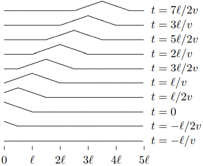
Figure \( 10.2\): A triangular pulse propagating on a stretched string.

Fourier integrals

Let us think about this problem in a more physical way. In the process, we will understand the physics of the general solution, (10.3). This may seem like a strange thing to say in a section entitled, “Fourier integrals.” Nevertheless, we will see that the mathematics of Fourier integrals has a direct and simple physical interpretation.

The idea is to use linearity in a clever way to solve this problem. We can take \(f(t)\) apart into its component angular frequencies. We already know how to solve the forced oscillation problem for each angular frequency. We can then take the individual solutions and add them back up again to reconstruct the solution to the full problem. The advantage of this procedure is that it works for any dispersion relation, not just for (10.1).

Because there may be a continuous distribution of frequencies in an arbitrary signal, we cannot just write \(f(t)\) as a sum over components, we need a Fourier integral, \[f(t)=\int_{-\infty}^{\infty} d \omega C(\omega) e^{-i \omega t} .\]

The physics of (10.9) is just linearity and time translation invariance. We know that we can choose the normal modes of the free system to have irreducible exponential time dependence, because of time translation invariance. Since the normal modes describe all the possible motions of the system, we know that by taking a suitable linear combination of normal modes, we can find a solution in which the motion of the end of the system is described by the function, \(f(t)\). The only subtlety in (10.9) is that we have assumed that the values of \(\omega\) that appear in the integral are all real. This is appropriate because a nonzero imaginary part for \(\omega\) in \(e^{-i \omega t}\) describes a function that goes exponentially to infinity as \(t \rightarrow \pm \infty\). Physically, we are never interested in such things. In fact, we are really interested in functions that go to zero as \(t \rightarrow \pm \infty\). These are well-described by the integral over real \(\omega\), (10.9).

Note that if \(f(t)\) is real in (10.9), then \[\begin{gathered}
f(t)=\int_{-\infty}^{\infty} d \omega C(\omega) e^{-i \omega t} \\
=f(t)^{*}=\int_{-\infty}^{\infty} d \omega C(\omega)^{*} e^{i \omega t}=\int_{-\infty}^{\infty} d \omega C(-\omega)^{*} e^{-i \omega t}
\end{gathered}\]

thus \[C(-\omega)^{*}=C(\omega) .\]

It is actually easier to work with the complex Fourier integral, (10.9), with the irreducible complex exponential time dependence, than with real expansions in terms of \(\cos \omega t\) and \(\sin \omega t\). But you may also see the real forms in other books. You can always translate from (10.9) by using the Euler identity \[e^{i \theta}=\cos \theta+i \sin \theta .\]

For each value of \(\omega\), we can write down the solution to the forced oscillation problem, incorporating the boundary condition at \(\infty\). Each frequency component of the force produces a wave traveling in the \(+x\) direction. \[e^{-i \omega t} \rightarrow e^{-i \omega t+i k x} ,\]

then we can use linearity to construct the solution by adding up the individual traveling waves from (10.13) with the coefficients \(C(\omega)\) from (10.9). Thus \[\psi(x, t)=\int_{-\infty}^{\infty} d \omega C(\omega) e^{-i \omega t+i k x} .\]

where \(\omega\) and \(k\) are related by the dispersion relation.

Equation (10.14) is true quite generally for any one-dimensional system, for any dispersion relation, but the result is particularly simple for a nondispersive system such as the continuous string with a dispersion relation of the form (10.1). We can use (10.1) in (10.14) by replacing \[k \rightarrow \omega / v .\]

Note that while \(k^{2}\) is determined by the dispersion relation, the sign of \(k\), for a given \(\omega\), is determined by the boundary condition at infinity. \(k\) and \(\omega\) must have the same sign, as in (10.15), to describe a wave traveling in the \(+x\) direction. Putting (10.15) into (10.14) gives \[\psi(x, t)=\int_{-\infty}^{\infty} d \omega C(\omega) e^{-i \omega t+i \omega x / v}=\int_{-\infty}^{\infty} d \omega C(\omega) e^{-i \omega(t-x / v)} .\]

Comparing this with (10.9) gives (10.7).

Let us try to understand what is happening in words. The Fourier integral, (10.9), expresses the signal as a linear combination of harmonic traveling waves. The relation, (10.15), which follows from the dispersion relation, (10.1), and the boundary condition at \(\infty\), implies that each of the infinite harmonic traveling waves moves at the same phase velocity. Therefore, the waves stay in exactly the same relationship to one another as they move, and the signal is never distorted. It just moves with the waves.

The nonharmonic signal is called a “wave packet.” As we have seen, it can be taken apart into harmonic waves, by means of the Fourier integral, (10.9).