10.2: Dispersive Media and Group Velocity

For any other dispersion relation, the signal changes shape as it propagates, because the various harmonic components travel at different velocities. Eventually, the various pieces of the signal get out of phase and the signal is dispersed. That is why such a medium is called “dispersive.” This is the origin of the name “dispersion relation.”

Group Velocity

10-2
If you are clever, you can send signals in a dispersive medium. The trick is to send the signal not directly as the function, \(f(t)\), but as a modulation of a harmonic signal, of the form \[f(t)=f_{s}(t) \cos \omega_{0} t ,\]

where \(f_{s}(t)\) is the signal. Very often, you want to do this anyway, because the important frequencies in your signal may not match the frequencies of the waves with which you want to send the signal. An example is AM radio transmission, in which the signal is derived from sound with a typical frequency of a few hundred cycles per second (Hz), but it is carried as a modulation of the amplitude of an electromagnetic radio wave, with a frequency of a few million cycles per second.¹

You can get a sense of what is going to happen in this case by considering the sum of two traveling waves with different frequencies and wave numbers, \[\cos \left(k_{+} x-\omega_{+} t\right)+\cos \left(k_{-} x-\omega_{-} t\right)\]

where \[k_{\pm}=k_{0} \pm k_{s}, \quad \omega_{\pm}=\omega_{0} \pm \omega_{s} ,\]

for \[k_{s} \ll k_{0}, \quad \omega_{s} \ll \omega_{0} .\]

The sum can be written as a product of cosines, as \[2 \cos \left(k_{s} x-\omega_{s} t\right) \cdot \cos \left(k_{0} x-\omega_{0} t\right) .\]

Because of (10.20), the first factor varies slowly in \(x\) and \(t\) compared to the second. The result can be thought of as a harmonic wave with frequency \(\omega_{0}\) with a slowly varying amplitude proportional to the first factor. The space dependence of (10.21) is shown in Figure \( 10.3\).

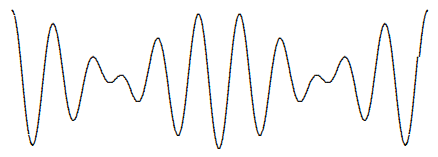
Figure \( 10.3\): The function (10.21) for t = 0 and k0/ks = 10.

You should think of the first factor in (10.21) as the signal. The second factor is called the “carrier wave.” Then (10.21) describes a signal that moves with velocity\[v_{s}=\frac{\omega_{s}}{k_{s}}=\frac{\omega_{+}-\omega_{-}}{k_{+}-k_{-}} ,\]

while the smaller waves associated with the second factor move with velocity \[v_{0}=\frac{\omega_{0}}{k_{0}} .\]

These two velocities will not be the same, in general. If (10.20) is satisfied, then (as we will show in more detail below) \(v_{0}\) will be roughly the phase velocity. In the limit, as \(k_{+}-k_{-}=2 k_{s}\) becomes very small, (10.22) becomes a derivative \[v_{s}=\left.\frac{\omega_{+}-\omega_{-}}{k_{+}-k_{-}} \rightarrow \frac{\partial \omega}{\partial k}\right|_{k=k_{0}} .\]

This is called the “group velocity.” It measures the speed at which the signal can actually be sent.

The time dependence of (10.21) is animated in program 10-2. Note the way that the carrier waves move through the signal. In this animation, the group velocity is smaller than the phase velocity, so the carrier waves appear at the back of each pulse of the signal and move through to the front.

Let us see how this works in general for interesting signals, \(f(t)\). Suppose that for some range of frequencies near some frequency \(\omega_{0}\), the dispersion relation is slowly varying. Then we can take it to be approximately linear by expanding \(\omega (k)\) in a Taylor series about \(k_{0}\) and keeping only the first two terms. That is \[\omega=\omega(k)=\omega_{0}+\left.\left(k-k_{0}\right) \frac{\partial \omega}{\partial k}\right|_{k=k_{0}}+\cdots,\]

\[\omega_{0} \equiv \omega\left(k_{0}\right),\]

and the higher order terms are negligible for a range of frequencies \[\omega_{0}-\Delta \omega<\omega<\omega_{0}+\Delta \omega .\]

where \(\Delta \omega\) is a constant that depends on \(\omega_{0}\) and the details on the higher order terms. Then you can send a signal of the form \[f(t) \cdot e^{-i \omega_{0} t}\]

(a complex form of (10.17), above) where \(f(t)\) satisfies (10.9) with \[C(\omega) \approx 0 \text { for }\left|\omega-\omega_{0}\right|>\Delta \omega .\]

This describes a signal that has a carrier wave with frequency \(\omega_{0}\), modulated by the interesting part of the signal, \(f(t)\), that acts like a time-varying amplitude for the carrier wave, \(e^{-i \omega_{0} t}\). The strategy of sending a signal as a varying amplitude on a carrier wave is called amplitude modulation.

Usually, the higher order terms in (10.25) are negligible only if \(\Delta \omega \ll \omega_{0}\). If we neglect them, we can write (10.25) as \[\omega=v k+a, \quad k=\omega / v+b,\]

where \(a\) and \(b\) are constants we can determine from (10.25), \[a=\omega_{0}-v k_{0}, \quad b=k_{0}-\omega_{0} / v\]

and \(v\) is the group velocity \[v=\left.\frac{\partial \omega}{\partial k}\right|_{k=k_{0}} .\]

For the signal (10.28) \[\psi(0, t)=\int_{-\infty}^{\infty} d \omega C(\omega) e^{-i\left(\omega+\omega_{0}\right) t}=\int_{-\infty}^{\infty} d \omega C\left(\omega-\omega_{0}\right) e^{-i \omega t} .\]

Thus (10.14) becomes \[\psi(x, t)=\int_{-\infty}^{\infty} d \omega C\left(\omega-\omega_{0}\right) e^{-i \omega t} e^{i k x} ,\]

but then (10.29) gives \[\begin{aligned}
\psi(x, t) &=\int_{-\infty}^{\infty} d \omega C\left(\omega-\omega_{0}\right) e^{-i \omega t+i(\omega / v+b) x} \\
=& \int_{-\infty}^{\infty} d \omega C\left(\omega-\omega_{0}\right) e^{-i \omega(t-x / v)+i b x} \\
=& \int_{=\infty}^{\infty} d \omega C(\omega) e^{-i\left(\omega+\omega_{0}\right)(t-x / v)+i b x} \\
&=f(t-x / v) e^{-i \omega_{0}(t-x / v)+i b x} .
\end{aligned}\]

The modulation \(f(t)\) travels without change of shape at the group velocity \(v\) given by (10.32), as long as we can ignore the higher order term in the dispersion relation. The phase velocity \[v_{\phi}=\frac{\omega}{k},\]

has nothing to do with the transmission of information, but notice that because of the extra \(e^{i b x}\) in (10.35), the carrier wave travels at the phase velocity.

You can see the difference between phase velocity and group velocity in your pool or bathtub by making a wave packet consisting of several shorter waves.

_________________
¹See (10.71), below.