17.7: Sample problems and solutions

Exercise \(\PageIndex{1}\)

Consider a charged sphere of radius, \(R\), which has a non-uniform charge density, that varies with radius, as \(\rho(r) = ar^2\).

1. What is the total charge on the sphere?
2. What is the electric field as a function of distance from the center of the sphere outside the sphere, \(r>R\)?
3. What is the electric field as a function of distance from the center of the sphere inside the sphere, \(r\leq R\)?

Answer

a. In order to determine the total charge of the sphere, we divide the sphere into infinitesimal shells of radius \(r\), and thickness, \(dr\). The volume, \(dV\), of one of these infinitesimal shells is their area (given by the area of the surface of a sphere of radius \(r\)), multiplied by their thickness, \(dr\):

\[\begin{aligned} dV = 4\pi r^2 dr\end{aligned}\]

The charge, \(dQ\), of one of those shells is given by the charge per unit volume, \(\rho(r)\):

\[\begin{aligned} dQ = \rho(r) dV = ar^24\pi r^2 dr = 4a\pi r^4 dr\end{aligned}\]

The total charge of the sphere is found by summing the charge from each shell:

\[\begin{aligned} Q=\int dQ =\int_0^R4a\pi r^4 dr=\frac{4}{5}a\pi R^5\end{aligned}\]

b. Outside of the sphere, we can use a spherical gaussian surface of radius \(r\), so that the flux is given by:

\[\begin{aligned} \oint \vec E\cdot d\vec A=4\pi r^2 E\end{aligned}\]

The entire charge of the sphere is enclosed. Applying Gauss’ Law, we can determine the electric field outside the sphere:

\[\begin{aligned} \oint \vec E\cdot d\vec A&= \frac{Q^{enc}}{\epsilon_0}\\[4pt] 4\pi r^2 E&= \frac{4a\pi R^5}{5\epsilon_0}\\[4pt] \therefore E(r)&=\frac{aR^5}{5\epsilon_0r^2}\end{aligned}\]

and we see that the electric field decreases as the radius squared, which makes sense, since from outside the sphere, we do not know how the charge is distributed within.

c. Inside the volume of the sphere, we still use a gaussian spherical surface of radius, \(r\), so that the flux is given by:

\[\begin{aligned} \oint \vec E\cdot d\vec A=4\pi r^2 E\end{aligned}\]

However, inside the sphere, the gaussian surface only encloses the charge up to a radius of \(r\), which we find by integration, similar to part a):

\[\begin{aligned} Q^{enc}=\int dQ =\int_0^r 4a\pi r^4 dr=\frac{4}{5}a\pi r^5\end{aligned}\]

Applying Gauss’ Law:

\[\begin{aligned} \oint \vec E\cdot d\vec A&= \frac{Q^{enc}}{\epsilon_0}\\[4pt] 4\pi r^2 E&= \frac{4a\pi r^5}{5\epsilon_0}\\[4pt] \therefore E(r)&=\frac{ar^3}{5\epsilon_0r^2}\end{aligned}\]

and we find that the electric field is zero at the center of the sphere and increases with radius cube inside the sphere.

Exercise \(\PageIndex{2}\)

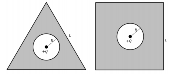
Consider two conducting plates which are illustrated in Figure \(\PageIndex{1}\). Both plates have a hollow circle of radius, \(R\), at their center. One plate is a square on the outside and the other is a triangle on the outside, both of the outside shapes have a side length of \(L\). A point charge of charge \(+Q\) is placed at the center of the hollowed out circle of both plates.

1. What is the electric field outside of the shells?
2. What is the average linear charge density on the inner and outer surfaces of the shells?
3. Which sections of the two plates would have the largest charge density?

Figure \(\PageIndex{1}\): A triangular and square shell, both with a hollowed out circular center and a point charge.

Answer

a. The conducting shells have no net charge, so the only charge in the system is the point charge \(Q\). If we draw a spherical gaussian surface, the only enclosed charge will be \(Q\), and we can ignore the charges on the plates. The electric field is thus the field from a point charge:

\[\begin{aligned} E= \frac{kQ}{r^2} \end{aligned}\]

b. Let’s begin with the shell that has a triangle on the outside. We will use Gauss’ law to determine the charge density of the inner and outer shells. To do this, we will draw a circle within the shell, \(S_1\) and a triangle outside of the outer shell, \(S_2\) as shown in Figure \(\PageIndex{2}\).

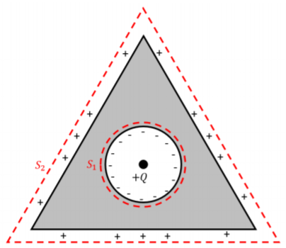
Figure \(\PageIndex{2}\): A solution to the triangular conducting shell.

When considering \(S_1\), we know that the electric field inside of the (conducting) shell is \(0\), so that the flux out of \(S_1\) will be zero. This means that the point charge on the inside of the shell will be equal and opposite to the sum of the surface charges on the inner shell. From here, we divide the net charge by the circumference of the inner shell to determine the linear charge density:

\[\begin{aligned} \lambda_{circle} = \frac{-Q}{2\pi R} \end{aligned}\]

When considering \(S_2\), we know that the \(Q_{enc} = +Q\), which means that the total linear charge on the outer triangle will be \(+Q\) such that it cancels the \(-Q\) along the inner circle. The sum of charges would be \(Q_{enc} = Q_{point}+Q_{triangle}-Q_{circle}\). Knowing this, we must divide the total charge on the outer surface by the sum of the length of each of the triangle’s sides in order to find the average linear charge density:

\[\begin{aligned} \lambda_{circle} = \frac{Q}{3L} \end{aligned}\]

Now, we consider the inner and outer linear charge densities of the square conducting shell. We choose two gaussian surfaces, \(S_1\), and \(S_2\), as shown in Figure \(\PageIndex{3}\):

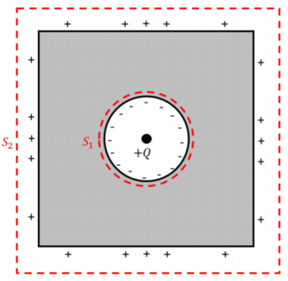
Figure \(\PageIndex{3}\): A solution to the square conducting shell.

For \(S_1\), the circle is treated as it was while solving the triangular shell. The electric field is also \(0\) within the square conducting shell, so we know that the average linear charge density is \(\frac{-Q}{2\pi R}\).

When considering \(S_2\), we know that \(Q_{enc}\) is \(+Q\), so we know that the total charge on the square surface of the shell will be \(+Q\). This leave us with the following average linear charge density:

\[\begin{aligned} \lambda_{square} = \frac{Q}{4L} \end{aligned}\]

c. These plates are charged by the electric field generated by the point charge held within them, which means that the linear charge density of the two plates will be highest at the points along the outer sides which are the shortest distance from the point charge. These points occur in the triangular and square plates at the point which is the closest to the charge, \(Q\), as shown in Figure \(\PageIndex{4}\).

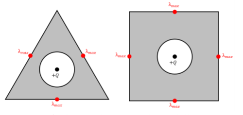
Figure \(\PageIndex{4}\): A solution to the square conducting shell.