

1.1: Position and Velocity
- Page ID
- 166606

\( \newcommand{\vecs}[1]{\overset { \scriptstyle \rightharpoonup} {\mathbf{#1}} } \)
\( \newcommand{\vecd}[1]{\overset{-\!-\!\rightharpoonup}{\vphantom{a}\smash {#1}}} \)
\( \newcommand{\dsum}{\displaystyle\sum\limits} \)
\( \newcommand{\dint}{\displaystyle\int\limits} \)
\( \newcommand{\dlim}{\displaystyle\lim\limits} \)
\( \newcommand{\id}{\mathrm{id}}\) \( \newcommand{\Span}{\mathrm{span}}\)
( \newcommand{\kernel}{\mathrm{null}\,}\) \( \newcommand{\range}{\mathrm{range}\,}\)
\( \newcommand{\RealPart}{\mathrm{Re}}\) \( \newcommand{\ImaginaryPart}{\mathrm{Im}}\)
\( \newcommand{\Argument}{\mathrm{Arg}}\) \( \newcommand{\norm}[1]{\| #1 \|}\)
\( \newcommand{\inner}[2]{\langle #1, #2 \rangle}\)
\( \newcommand{\Span}{\mathrm{span}}\)
\( \newcommand{\id}{\mathrm{id}}\)
\( \newcommand{\Span}{\mathrm{span}}\)
\( \newcommand{\kernel}{\mathrm{null}\,}\)
\( \newcommand{\range}{\mathrm{range}\,}\)
\( \newcommand{\RealPart}{\mathrm{Re}}\)
\( \newcommand{\ImaginaryPart}{\mathrm{Im}}\)
\( \newcommand{\Argument}{\mathrm{Arg}}\)
\( \newcommand{\norm}[1]{\| #1 \|}\)
\( \newcommand{\inner}[2]{\langle #1, #2 \rangle}\)
\( \newcommand{\Span}{\mathrm{span}}\) \( \newcommand{\AA}{\unicode[.8,0]{x212B}}\)
\( \newcommand{\vectorA}[1]{\vec{#1}} % arrow\)
\( \newcommand{\vectorAt}[1]{\vec{\text{#1}}} % arrow\)
\( \newcommand{\vectorB}[1]{\overset { \scriptstyle \rightharpoonup} {\mathbf{#1}} } \)
\( \newcommand{\vectorC}[1]{\textbf{#1}} \)
\( \newcommand{\vectorD}[1]{\overrightarrow{#1}} \)
\( \newcommand{\vectorDt}[1]{\overrightarrow{\text{#1}}} \)
\( \newcommand{\vectE}[1]{\overset{-\!-\!\rightharpoonup}{\vphantom{a}\smash{\mathbf {#1}}}} \)
\( \newcommand{\vecs}[1]{\overset { \scriptstyle \rightharpoonup} {\mathbf{#1}} } \)
\(\newcommand{\longvect}{\overrightarrow}\)
\( \newcommand{\vecd}[1]{\overset{-\!-\!\rightharpoonup}{\vphantom{a}\smash {#1}}} \)
\(\newcommand{\ket}[1]{\left| #1 \right>}\)
\(\newcommand{\bra}[1]{\left< #1 \right|}\)
\(\newcommand{\braket}[2]{\left< #1 \vphantom{#2} \right| \left. #2 \vphantom{#1} \right>}\)
\(\newcommand{\braopket}[3]{\left< #1 \vphantom{#2}\vphantom{#3} \right| #2 \vphantom{#1}\vphantom{#3} \left| #3 \vphantom{#1}\vphantom{#2} \right>}\)
\(\newcommand{\qmvec}[1]{\mathbf{\vec{#1}}}\)
\(\newcommand{\op}[1]{\hat{\mathbf{#1}}}\)
\(\newcommand{\expect}[1]{\langle #1 \rangle}\)
\(\newcommand{\dfn}[1]{\emph{\textbf{#1}}}\)
Standard practiced: K1 (motion maps and motion graphs). This activity builds position and velocity on motion maps. The next activity adds changing velocity.
A motion map shows only positions: one dot for each photo of an object, labeled with its clock reading. In this workbook, the photos are always 1 second apart. You will mark up the motion map with arrows to show changes in position and velocity.
Whiteboard first: in class, your group drafts its key work on the whiteboard. When the group agrees, everyone copies the final version into their notes.
Colors: use 3 or 4 colors to highlight. Using the same color for the same quantity in a diagram and in an equation shows where that quantity appears in each.
Before class: complete each Explore section on your own. Every Explore answer can be found in the Model above it.
The kinematics model. In every kinematics activity, "Model the scenario" means building these parts so that each one agrees with the others:
- Physical story: what happens, in words, with a positive direction chosen.
- Motion map: positions at equal time intervals, marked up with change in position, velocity, and change in velocity arrows.
- Graphs: position, velocity, and acceleration against clock reading.
- Equations: update equations (initial + change = final), and later, functions grouped by powers of t.
- Math solution: circle each unknown, solve, and check the answer against the other parts.
This activity builds the physical story, the motion map, and the update equations. Later activities add the other parts.
1. Where and When
 Model
Physical story
Two delivery robots roll along a straight sidewalk, each at a steady pace. A camera above the sidewalk takes a photo every second. Positions are measured from a crack in the sidewalk, and to the right is positive.
Motion map
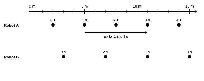
Position at a clock reading
means Robot A's position at the clock reading 1 s is 5 m.
Initial, final, and change
An interval runs from one clock reading to a later one. Robot A's position at the start of the interval is its initial position, . Its position at the end is its final position, . Its change in position, or displacement, , is an arrow from the initial dot to the final dot. An arrow to the right is positive, and an arrow to the left is negative.
| Interval | Initial position | Final position | Change in position |
|---|---|---|---|
| Robot A, 1 s to 3 s | |||
| Robot A, 0 s to 2 s | |||
| Robot A, 2 s to 4 s | |||
| Robot B, 1 s to 3 s |
 Explore
- Find each position: Robot A at 0 s, Robot A at 4 s, and Robot B at 2 s. Write each one like .
- For the interval 2 s to 4 s, which clock reading gives the initial position and which gives the final position? How do you know?
- Complete the table in the Model. For each row, mark the Δx arrow on the motion map, from the initial dot to the final dot, and label its length.
 Critical thinking & Concept Invention
Launch: Manager, read the physical story aloud. Then have each person point to one dot and say the position and clock reading, like "x of 1 second is 5 meters."
Compare: Check your table and Δx arrows with your group.
- Highlight Robot A's initial position, change in position, and final position for 1 s to 3 s in three colors, in the table and on the motion map (initial dot, arrow, final dot). Then answer on your whiteboard: how do you find a final position if you know the initial position and the change? Write your answer in words, then as an equation using , , and . Check it on every row of the table, and highlight its terms in the same three colors. Finalize it on your whiteboard as a group, then copy it into your notes below.
- Robot B's Δx arrow from 1 s to 3 s is 8 m long, but its change in position is −8 m. Does your equation still work for Robot B? What does the sign of Δx tell you? Finalize it on your whiteboard as a group, then copy it into your notes below.
- On your whiteboard, rearrange your equation to find the change in position from the initial and final positions. Use it to find Robot A's change in position from 0 s to 4 s, then check your answer with an arrow on the motion map. Finalize it on your whiteboard as a group, then copy it into your notes below.
- A group member writes . Is this the same equation as yours? Which term is the initial position, and which is the final? Write the same kind of equation for Robot B from 0 s to 3 s, with numbers.
+ =
- A group member says that Robot B's change in position from 0 s to 3 s must be positive, because its final position, 3 m, is positive. Write the Claim, Evidence, Reasoning template on your whiteboard and answer the question: do you agree? Finalize it on your whiteboard as a group, then copy it into your notes below.
Claim
Evidence
Reasoning
Check in: Reflector, check that everyone can explain how to find a final position from an initial position and a change. Set your cup.
2. How Fast and Which Way
Model
These are the same two robots from Part 1. Each robot rolls at a steady pace.

Time interval
The time interval, , is the final clock reading minus the initial clock reading. From 1 s to 3 s, .
Robot A
| Interval | Δx | Δt | Δx/Δt |
|---|---|---|---|
| 0 s to 1 s | |||
| 1 s to 2 s | |||
| 0 s to 2 s | |||
| 1 s to 4 s | |||
| 0 s to 4 s |
Explore
- Complete Robot A's table in the Model. Use the motion map or your equation from Part 1 to find each Δx.
- Which interval has the largest Δx? Which has the largest Δx/Δt?
Critical thinking & Concept Invention
Launch: Manager, have each person say one Δx/Δt value from the table and its interval.
- What do you notice about Δx/Δt for Robot A? On your whiteboard, use the spacing of the dots on the motion map to explain why. Finalize it on your whiteboard as a group, then copy it into your notes below.
- The ratio Δx/Δt tells how far and which way an object moves per second. It is called the velocity: . On your whiteboard, make a Δx, Δt, and Δx/Δt table for Robot B, using three intervals of your choice. What is Robot B's velocity, with its sign? Finalize it on your whiteboard as a group, then copy it into your notes below.
- Mark velocity arrows on the motion map: just below each dot, draw that robot's velocity arrow, using 1 m on the ruler for each 1 m/s. On your whiteboard, compare a velocity arrow with Robot A's Δx arrow for a 1 s interval, and with its Δx arrow for a 2 s interval. Finalize it on your whiteboard as a group, then copy it into your notes below.
- A group member says Robot B's velocity (−4 m/s) is smaller than Robot A's velocity (+3 m/s), because −4 is less than 3. Write the Claim, Evidence, Reasoning template on your whiteboard and answer the question: do you agree? Finalize it on your whiteboard as a group, then copy it into your notes below.
Claim
Evidence
Reasoning
- How can you find Δx if you know the velocity and the time interval? On your whiteboard, answer that, then put it into your position update equation from Part 1. Use your new equation to find Robot A's position at 10 s and the clock reading when Robot B reaches 0 m. Circle each unknown. Finalize it on your whiteboard as a group, then copy it into your notes below.
Check in: Reflector, check that everyone can explain why Δx/Δt is the same for every interval of Robot A. Set your cup.
3. When the Pace Changes
Model
Physical story
A third delivery robot makes a delivery. It speeds up, slows down to stop at a doorstep for a moment, then starts back. The camera still takes a photo every second, and to the right is positive.
Motion map

| Interval | Δx | Δt | Δx/Δt |
|---|---|---|---|
| 0 s to 1 s | |||
| 1 s to 2 s | |||
| 0 s to 2 s | |||
| 0 s to 4 s | |||
| 4 s to 5 s | |||
| 4 s to 6 s |
Explore
- Mark a Δx arrow on the motion map for each second, and label its length. If the robot did not move, write 0 instead of drawing an arrow.
- Complete the table in the Model.
Critical thinking & Concept Invention
Launch: Manager, read the physical story aloud. Then have each person point to a part of the motion map where the robot was fast, slow, or at rest.
Compare: Check your table with your group.
- Is Δx/Δt the same for every interval of this robot? On your whiteboard, explain what is different about this motion map compared with Robot A's. Finalize it on your whiteboard as a group, then copy it into your notes below.
- When the velocity changes, Δx/Δt for an interval is the average velocity for that interval: . From 0 s to 4 s, the average velocity is +3 m/s. Does +3 m/s describe the robot's motion from 0 s to 1 s? On your whiteboard, decide which intervals describe the robot's motion best, moment by moment, and explain. Finalize it on your whiteboard as a group, then copy it into your notes below.
- From 0 s to 6 s, the robot rolled 12 m out and 3 m back, 15 m in all. A group member says its average velocity from 0 s to 6 s was (15 m)/(6 s) = 2.5 m/s. Write the Claim, Evidence, Reasoning template on your whiteboard and answer the question: do you agree? Finalize it on your whiteboard as a group, then copy it into your notes below.
Claim
Evidence
Reasoning
- Use the average velocity from 0 s to 4 s and to predict the robot's position at 1 s. Compare it with the motion map. On your whiteboard, explain when this equation gives the right position for any time interval. Finalize it on your whiteboard as a group, then copy it into your notes below.
Check in: Reflector, check that everyone can explain the difference between velocity and average velocity. Set your cup.
 Summary
- A motion map shows positions, one dot per clock reading. is the position at the clock reading 1 s. For an interval, the earlier reading gives the initial position and the later one gives the final position.
- The change in position, Δx, is an arrow from the initial dot to the final dot. Its sign shows its direction. The position update equation and its rearranged form are
- Velocity is the change in position per time, . When the dots are equally spaced, the velocity is constant, and Δx/Δt is the same for every interval. The length of a velocity arrow is the speed, and in one dimension the sign shows the direction.
- With a constant velocity, works for any time interval.
- When the velocity changes, Δx/Δt is the average velocity for that interval. Shorter intervals describe the motion better. Average velocity uses the change in position, not the total distance.
- Update equations follow one pattern: final = initial + change. You will use this pattern for velocity in the next activity, and for momentum later in the course.
 Apply
Build each piece on your whiteboard, finalize it as a group, then copy it into your notes before starting the next piece.
- Model the scenario. A skateboarder starts at 4 m and rolls at +3 m/s for 2 s, stops for 1 s, then rolls back at −2 m/s for 3 s. Draw the motion map, with a dot for each second. Then mark a Δx arrow for each second. Write a position update equation to find the skateboarder's position at 6 s, and circle the unknown.

- The skateboarder's average velocity from 0 s to 6 s is 0 m/s. A friend says that means the skateboarder never moved. Write the Claim, Evidence, Reasoning template on your whiteboard and answer the question: do you agree? Finalize it on your whiteboard as a group, then copy it into your notes below.
Claim
Evidence
Reasoning
Check in: Reflector, before the consensus share-out, check that your group agrees on both answers.