

1.2: Kinematics Graphs
- Page ID
- 166607

\( \newcommand{\vecs}[1]{\overset { \scriptstyle \rightharpoonup} {\mathbf{#1}} } \)
\( \newcommand{\vecd}[1]{\overset{-\!-\!\rightharpoonup}{\vphantom{a}\smash {#1}}} \)
\( \newcommand{\dsum}{\displaystyle\sum\limits} \)
\( \newcommand{\dint}{\displaystyle\int\limits} \)
\( \newcommand{\dlim}{\displaystyle\lim\limits} \)
\( \newcommand{\id}{\mathrm{id}}\) \( \newcommand{\Span}{\mathrm{span}}\)
( \newcommand{\kernel}{\mathrm{null}\,}\) \( \newcommand{\range}{\mathrm{range}\,}\)
\( \newcommand{\RealPart}{\mathrm{Re}}\) \( \newcommand{\ImaginaryPart}{\mathrm{Im}}\)
\( \newcommand{\Argument}{\mathrm{Arg}}\) \( \newcommand{\norm}[1]{\| #1 \|}\)
\( \newcommand{\inner}[2]{\langle #1, #2 \rangle}\)
\( \newcommand{\Span}{\mathrm{span}}\)
\( \newcommand{\id}{\mathrm{id}}\)
\( \newcommand{\Span}{\mathrm{span}}\)
\( \newcommand{\kernel}{\mathrm{null}\,}\)
\( \newcommand{\range}{\mathrm{range}\,}\)
\( \newcommand{\RealPart}{\mathrm{Re}}\)
\( \newcommand{\ImaginaryPart}{\mathrm{Im}}\)
\( \newcommand{\Argument}{\mathrm{Arg}}\)
\( \newcommand{\norm}[1]{\| #1 \|}\)
\( \newcommand{\inner}[2]{\langle #1, #2 \rangle}\)
\( \newcommand{\Span}{\mathrm{span}}\) \( \newcommand{\AA}{\unicode[.8,0]{x212B}}\)
\( \newcommand{\vectorA}[1]{\vec{#1}} % arrow\)
\( \newcommand{\vectorAt}[1]{\vec{\text{#1}}} % arrow\)
\( \newcommand{\vectorB}[1]{\overset { \scriptstyle \rightharpoonup} {\mathbf{#1}} } \)
\( \newcommand{\vectorC}[1]{\textbf{#1}} \)
\( \newcommand{\vectorD}[1]{\overrightarrow{#1}} \)
\( \newcommand{\vectorDt}[1]{\overrightarrow{\text{#1}}} \)
\( \newcommand{\vectE}[1]{\overset{-\!-\!\rightharpoonup}{\vphantom{a}\smash{\mathbf {#1}}}} \)
\( \newcommand{\vecs}[1]{\overset { \scriptstyle \rightharpoonup} {\mathbf{#1}} } \)
\(\newcommand{\longvect}{\overrightarrow}\)
\( \newcommand{\vecd}[1]{\overset{-\!-\!\rightharpoonup}{\vphantom{a}\smash {#1}}} \)
\(\newcommand{\ket}[1]{\left| #1 \right>}\)
\(\newcommand{\bra}[1]{\left< #1 \right|}\)
\(\newcommand{\braket}[2]{\left< #1 \vphantom{#2} \right| \left. #2 \vphantom{#1} \right>}\)
\(\newcommand{\braopket}[3]{\left< #1 \vphantom{#2}\vphantom{#3} \right| #2 \vphantom{#1}\vphantom{#3} \left| #3 \vphantom{#1}\vphantom{#2} \right>}\)
\(\newcommand{\qmvec}[1]{\mathbf{\vec{#1}}}\)
\(\newcommand{\op}[1]{\hat{\mathbf{#1}}}\)
\(\newcommand{\expect}[1]{\langle #1 \rangle}\)
\(\newcommand{\dfn}[1]{\emph{\textbf{#1}}}\)
Standard practiced: K1 (motion maps and motion graphs). This activity connects motion maps to graphs. The K1 quiz covers this activity and Motion Maps: Position and Velocity.
A graph of position or velocity against clock reading tells the same story as a motion map. In this activity, you will find the slopes and areas of graphs and connect them to the arrows on motion maps.
Whiteboard first: in class, your group drafts its key work on the whiteboard. When the group agrees, everyone copies the final version into their notes.
Colors: use 3 or 4 colors to highlight. Using the same color for the same quantity in a diagram and in an equation shows where that quantity appears in each.
Before class: complete each Explore section on your own. Every Explore answer can be found in the Model above it.
The kinematics model: physical story, motion map, graphs, equations, and math solution. This activity adds the graphs.
1. Position Graphs
 Model
These are the two delivery robots from Motion Maps: Position and Velocity. Robot A's positions are plotted on the position graph below.
Motion map

Position graph

The slope of a line is its rise over its run. On a position graph, the rise is a change in position, Δx, and the run is a time interval, Δt.
 Explore
- Use the graph to find Robot A's position at 2 s. Check it with the motion map.
- Find the rise (Δx) and the run (Δt) of the slope triangle. Highlight the Δx side of the triangle in one color, then draw Robot A's Δx arrow for 1 s to 3 s on the motion map and highlight it in the same color.
- Plot Robot B's positions on the position graph and connect them.
 Critical thinking & Concept Invention
Launch: Manager, have each person point to one dot on the graph and the matching dot on the motion map.
- On your whiteboard, find the slope of Robot A's line and the slope of Robot B's line, with units. What quantity does the slope of a position graph tell you? Then, connecting to calculus: is a slope a derivative or an integral, and of which quantity? Finalize it on your whiteboard as a group, then copy it into your notes below.
- A third robot is parked at 9 m the whole time. Draw its line on the graph. On your whiteboard, write a rule: how do the steepness and the direction of a line on a position graph show an object's velocity? Finalize it on your whiteboard as a group, then copy it into your notes below.
- At 3 s, Robot A's point is higher on the graph than Robot B's. A group member says that means Robot A is moving faster. Write the Claim, Evidence, Reasoning template on your whiteboard and answer the question: do you agree? Finalize it on your whiteboard as a group, then copy it into your notes below.
Claim
Evidence
Reasoning
Check in: Reflector, check that everyone can find a velocity from a position graph. Set your cup.
2. Velocity Graphs and Area
Model
Physical story
This is the skateboarder from Motion Maps: Position and Velocity. The skateboarder starts at 4 m, rolls at +3 m/s for 2 s, stops for 1 s, then rolls back at −2 m/s for 3 s.
Velocity graph

The area under a velocity graph is the area between the graph and the t axis. Area below the t axis counts as negative.
Position graph

Explore
- Use the velocity graph to find the skateboarder's velocity at 1 s and at 4 s.
- Find the shaded area, from 0 s to 2 s. Multiply the height by the width, and keep the units.
- Shade the rest of the area under the velocity graph, and find the area from 2 s to 3 s and from 3 s to 6 s.
Critical thinking & Concept Invention
Launch: Manager, read the physical story aloud. Then have each person say one area and its units.
Compare: Check your areas with your group.
- The skateboarder's Δx arrows from Motion Maps: Position and Velocity were 6 m right from 0 s to 2 s, 0 from 2 s to 3 s, and 6 m left from 3 s to 6 s. On your whiteboard, explain what the area under a velocity graph tells you. Use the units and the sign of the areas. Then, connecting to calculus: is an area under a graph a derivative or an integral, and of which quantity? Finalize it on your whiteboard as a group, then copy it into your notes below.
- On your whiteboard, write the position update equation using the area under the velocity graph. Use it to find the skateboarder's position at 2 s, 3 s, and 6 s, then draw the position graph in the Model. Highlight each area on the velocity graph and the matching rise on the position graph in the same color. Finalize it on your whiteboard as a group, then copy it into your notes below.
- A group member says the skateboarder's position at 5 s is negative, because the velocity graph is below the t axis at 5 s. Write the Claim, Evidence, Reasoning template on your whiteboard and answer the question: do you agree? Finalize it on your whiteboard as a group, then copy it into your notes below.
Claim
Evidence
Reasoning
Check in: Reflector, check that everyone can find a change in position from a velocity graph. Set your cup.
3. Changing Velocity and Acceleration
Model
Physical story
A car drives along a straight road. Its dashcam records the speedometer every second. The car speeds up, holds steady, then slows down for a crosswalk. East is positive. Between readings, assume the velocity changes steadily.
Motion map with velocity arrows

Each velocity arrow shows the speedometer reading at that instant, with its direction. Each change in velocity arrow, Δv, shows how the velocity changed during one second.
Velocity graph

Acceleration graph (to build)

Explore
- Complete the Δv arrows on the motion map. Label each one, and write 0 if the velocity did not change.
- Use the velocity graph to find Δv for each second. Highlight the Δv side of the slope triangle and the 0 s to 1 s Δv arrow on the motion map in the same color.
Critical thinking & Concept Invention
Launch: Manager, read the physical story aloud. Then have each person point to one part of the velocity graph where the car speeds up, holds steady, or slows down.
- The position update equation is . On your whiteboard, write a velocity update equation with the same pattern, using , , and . Check it on the velocity graph from 0 s to 1 s, then write it for 3 s to 4 s with numbers and signs. Finalize it on your whiteboard as a group, then copy it into your notes below.
+ =
- The slope of a velocity graph, the change in velocity per time, is called the acceleration: . Its units are (m/s)/s, written m/s². On your whiteboard, find the acceleration for each second. Then write a rule: how do the signs of the velocity and the acceleration tell you whether the car is speeding up or slowing down? Then, connecting to calculus: is the slope of a velocity graph a derivative or an integral, and of which quantity? Finalize it on your whiteboard as a group, then copy it into your notes below.
- From the motion map, the car's positions at 0 s to 5 s are 0, 5.5, 13.5, 22.5, 29.5, and 33 m. Plot them on the position graph below and connect them with a smooth curve. On your whiteboard, explain how the steepness of the curve shows the car speeding up, holding steady, and slowing down. Use the meaning of the slope of a position graph from Part 1. Then, connecting to calculus: is that slope a derivative or an integral, and of which quantity? Finalize it on your whiteboard as a group, then copy it into your notes below.

- On your whiteboard, build the acceleration graph: draw a flat segment for each second at that second's acceleration. Shade the area between each segment and the t axis. Finalize it on your whiteboard as a group, then copy it into your notes below. Then draw the graph in the Model.
- What does the area under the acceleration graph from 0 s to 2 s tell you? Find it, with units, and check your answer with the velocity graph. Then, connecting to calculus: is this area a derivative or an integral, and of which quantity?
Check in: Reflector, check that everyone can find an acceleration from a velocity graph. Set your cup.
4. Ball Toss
Model
Physical story
You toss a ball straight up at 10 m/s from the edge of a cliff. It rises, stops for an instant, then falls past you toward the beach below. A camera records the ball every second. Up is positive, and air resistance is small enough to ignore.
A note on g: in this course, we round the acceleration of a falling object near Earth's surface to 10 m/s². The measured value is closer to 9.8 m/s², and you may see 9.8 m/s² in other books, classes, and websites.
Motion map with velocity arrows

Velocity graph

The dashed lines mark the middle of each second.
Explore
- Use the motion map to find the ball's displacement, Δy, for each second. Then find the average velocity for each second, .
0 s to 1 s 1 s to 2 s 2 s to 3 s 3 s to 4 s Δy Average velocity - Use the velocity graph to find the ball's velocity at 1 s and at 2 s.
Critical thinking & Concept Invention
Launch: Manager, read the physical story aloud. Then have each person predict the ball's acceleration at its highest point.
Compare: Check your Explore table with your group.
- Plot each second's average velocity on the velocity graph, on the dashed line in the middle of that second. What do you notice? On your whiteboard, explain why the middle of the second is the right place to plot an average velocity when the velocity changes steadily. Finalize it on your whiteboard as a group, then copy it into your notes below.
- At 1 s, the ball's velocity is 0. A group member says the ball's acceleration must also be 0 at the top. Write the Claim, Evidence, Reasoning template on your whiteboard and answer the question: is the acceleration 0 at the top? Finalize it on your whiteboard as a group, then copy it into your notes below.
Claim
Evidence
Reasoning
- Shade the area under the velocity graph from 2 s to 3 s. Split it into a rectangle, with height , and a triangle, with height . On your whiteboard, write the area of each piece using , , and , then add them to write an equation for Δy. Check it against your Explore table. Then, connecting to calculus: is the area you found a derivative or an integral, and of which quantity? Finalize it on your whiteboard as a group, then copy it into your notes below.
- On your whiteboard, use your equation for Δy over the whole interval from 0 s to 4 s, then use the position update equation to find the ball's position at 4 s. Circle each unknown, and check your answer with the motion map. Finalize it on your whiteboard as a group, then copy it into your notes below.
Check in: Reflector, check that everyone can explain why the acceleration is not 0 at the top. Set your cup.
 Summary
- The slope of a position graph is the velocity. Steeper means faster, and a flat line means at rest.
- The area under a velocity graph is the change in position, Δx. Area below the t axis is negative. .
- The slope of a velocity graph is the acceleration, , in m/s². When the velocity and the acceleration have the same sign, the object speeds up. When they have opposite signs, it slows down.
- The area under an acceleration graph is the change in velocity, Δv. .
- When the velocity changes steadily, the average velocity for an interval equals the velocity at the middle of the interval, and (a rectangle plus a triangle).
- In calculus language, a slope is a derivative and an area is an integral: velocity is the derivative of position, acceleration is the derivative of velocity, Δx is the integral of velocity, and Δv is the integral of acceleration.
- Near Earth's surface, with air resistance ignored, a tossed or dropped object has an acceleration of about 10 m/s² downward, on the way up, at the top, and on the way down. We use 10 m/s² in this course; the measured value is closer to 9.8 m/s², which you may see elsewhere.
 Apply
Build each piece on your whiteboard, finalize it as a group, then copy it into your notes before starting the next piece. Write each equation with variables before you put in numbers.
- Model the scenario. A cart has an initial velocity of +3 m/s and an acceleration of −0.6 m/s². Sketch its velocity graph from 0 s to 3 s. Then find its velocity and its displacement at 3 s. Circle each unknown.
The cart starts at x = 0. Use the area under your velocity graph for each second to draw its motion map, with a dot for each second. Mark a velocity arrow at each dot and a change in velocity arrow for each second. Then sketch its position graph, and check that your motion map and position graph agree.
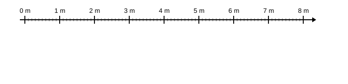

- Model the scenario. The graph shows the velocities of a car and a truck. Find the acceleration and the displacement of each from 0 s until it stops.
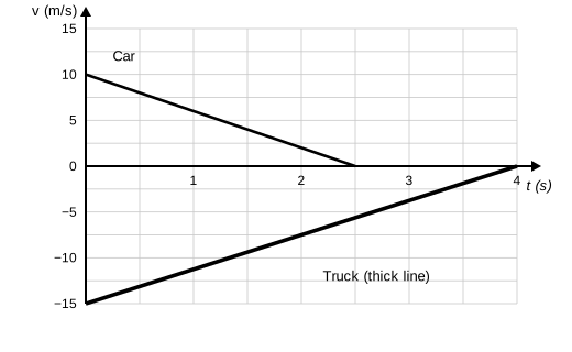
- A group member says the truck speeds up from 0 s to 4 s, because its acceleration is positive. Write the Claim, Evidence, Reasoning template on your whiteboard and answer the question: do you agree? Finalize it on your whiteboard as a group, then copy it into your notes below.
Claim
Evidence
Reasoning
Check in: Reflector, before the consensus share-out, check that your group agrees on all three answers.