2.4: Electrostatic Force - Coulomb's Law

Coulomb's Force

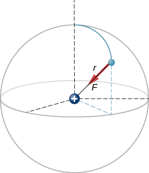
Experiments with electric charges have shown that if two objects each have electric charge, then they exert an electric force on each other. The magnitude of the force is linearly proportional to the net charge on each object and inversely proportional to the square of the distance between them. (Interestingly, the force does not depend on the mass of the objects.) The direction of the force vector is along the imaginary line joining the two objects and is dictated by the signs of the charges involved.

Let

• $q_1, q_2 =$ the net electric charge of the two objects;
• $\vec{r}_{12} =$ the vector displacement from $q_1$ to $q_2$.

The electric force $\vec{F}$ on one of the charges is proportional to the magnitude of its own charge and the magnitude of the other charge, and is inversely proportional to the square of the distance between them:

$$F \propto \dfrac{q_1q_2}{r_{12}^2}.$$

This proportionality becomes an equality with the introduction of a proportionality constant:

Coulomb's Law

The electric force (or Coulomb force) experienced by charge $q_2$ due to charge $q_1$ is equal to

$$\vec{F}_{12}=\frac{1}{4 \pi \varepsilon_{0}}\ \frac{q_{1}\ q_{2}}{r_{12}^{2}}\hat{r}_{12}=\frac{1}{4 \pi \varepsilon_{0}}\ \frac{q_{1}\ q_{2}}{r_{12}^{3}}\vec{r}_{12} \label{Coulomb}$$

The unit vector $\hat{r}_{12}=\frac{\vec{r}_{12}}{\left|\vec{r}_{12}\right|}$ has a magnitude of 1 and points along the axis as the charges from $q_1$ to $q_2$ (same direction as vector $\vec{r}_{12}$).

Figure: The vector $\vec{r}_{12}$ between point charges $q_1$ and $q_2$ .

If the charges have the same sign, the force is in the same direction as $\vec{r}_{12}$ showing a repelling force. If the charges have different signs, the force is in the opposite direction of $\vec{r}_{12}$ showing an attracting force. (Figure $\PageIndex{1}$).

Figure $\PageIndex{1}$: The electrostatic force $\vec{F}$ between point charges $q_1$ and $q_2$ separated by a distance $\left|\vec{r}_{12}\right|=\left|\vec{r}_{21}\right|$ is given by Coulomb’s law. Note that Newton’s third law (every force exerted creates an equal and opposite force) applies as usual—the force on $q_1$ is equal in magnitude and opposite in direction to the force it exerts on $q_2$ - $\vec{F}_{12}=-\vec{F}_{21}$. (a) Like charges; (b) unlike charges.

It is important to note that the electric force is not constant; it is a function of the separation distance between the two charges. If either the test charge or the source charge (or both) move, then $\vec{r}$ changes, and therefore so does the force. An immediate consequence of this is that direct application of Newton’s laws with this force can be mathematically difficult, depending on the specific problem at hand. It can (usually) be done, but we almost always look for easier methods of calculating whatever physical quantity we are interested in. (Conservation of energy is the most common choice.)

Finally, the new constant $\epsilon_0$ in Coulomb’s law is called the permittivity of free space, or (better) the permittivity of vacuum. It has a very important physical meaning that we will discuss in a later chapter; for now, it is simply an empirical proportionality constant. Its numerical value (to three significant figures) turns out to be

$$\epsilon_0 = 8.85 \times 10^{-12} \dfrac{\text{C}^2}{\text{N} \cdot \text{m}^2}.$$

These units are required to give the force in Coulomb’s law the correct units of newtons. Note that in Coulomb’s law, the permittivity of vacuum is only part of the proportionality constant. For convenience, we often define a Coulomb’s constant:

$$k_e = \dfrac{1}{4\pi \epsilon_0} = 8.99 \times 10^9 \dfrac{\text{N} \cdot \text{m}^2}{\text{C}^2}.$$

Examples 

Example $\PageIndex{1}$: The Force on the Electron in Hydrogen

A hydrogen atom consists of a single proton and a single electron. The proton has a charge of $+e$ and the electron has $-e$. In the “ground state” of the atom, the electron orbits the proton at most probable distance of $5.29 \times 10^{-11} \text{m}$ (Figure $\PageIndex{2}$). Calculate the electric force on the electron due to the proton.

Figure $\PageIndex{2}$: A schematic depiction of a hydrogen atom, showing the force on the electron. This depiction is only to enable us to calculate the force; the hydrogen atom does not really look like this.

Strategy

For the purposes of this example, we are treating the electron and proton as two point particles, each with an electric charge, and we are told the distance between them; we are asked to calculate the force on the electron. We thus use Coulomb’s law (Equation $\ref{Coulomb}$).

Solution

Our two charges are,

$$\begin{align*} q_1 &= +e \\[4pt] &= +1.602 \times 10^{-19} \text{C} \\[4pt] q_2 &= -e \\[4pt] &= -1.602 \times 10^{-19} \text{C} \end{align*}$$

and the distance between them

$$r = 5.29 \times 10^{-11} \text{m}. \nonumber$$

The magnitude of the force on the electron (Equation $\ref{Coulomb}$) is

$$\begin{align*} F &= \dfrac{1}{4\pi \epsilon_0}\dfrac{|q_1q_2|}{r_{12}^2} \\[4pt] &= \dfrac{1}{4\pi \left(8.85 \times 10^{-12} \frac{\text{C}^2}{ \text{N} \cdot \text{m}^2} \right)} \dfrac{(1.602 \times 10^{-19} \text{C})^2}{(5.29 \times 10^{-11} \text{m})^2} \\[4pt] &= 8.25 \times 10^{-8} \end{align*}$$

As for the direction, since the charges on the two particles are opposite, the force is attractive; the force on the electron points radially directly toward the proton, everywhere in the electron’s orbit. The force is thus expressed as

$$\vec{F} = - (8.25 \times 10^{-8} \text{N}) \hat{r}. \nonumber$$

Universal Gravitational Expression

You might have noticed that Coulomb's force bears a striking resemblance to the Universal Gravitational Expression between two masses $m_1$ and $m_2$

$$\vec{F}_{12}=-G\ \frac{m_{1}\ m_{2}}{r_{12}^{2}}\hat{r}_{12}=-G\ \frac{m_{1}\ m_{2}}{r_{12}^{3}}\vec{r}_{12} \label{Gravity}$$

 

Multiple Source Charges

The analysis that we have done for two particles can be extended to an arbitrary number of particles; we simply repeat the analysis, two charges at a time. Specifically, we ask the question: Given N charges (which we refer to as source charge), what is the net electric force that they exert on some other point charge (which we call the test charge)? Note that we use these terms because we can think of the test charge being used to test the strength of the force provided by the source charges.

Like all forces that we have seen up to now, the net electric force on our test charge is simply the vector sum of each individual electric force exerted on it by each of the individual test charges. Thus, we can calculate the net force on the test charge Q by calculating the force on it from each source charge, taken one at a time, and then adding all those forces together (as vectors). This ability to simply add up individual forces in this way is referred to as the principle of superposition, and is one of the more important features of the electric force. In mathematical form, this becomes

$$\vec{F}(r) = \dfrac{1}{4\pi \epsilon_0} Q \sum_{i=1}^N \dfrac{q_i}{r_i^2}\hat{r}_i^2. \label{sup}$$

In this expression, Q represents the charge of the particle that is experiencing the electric force $\vec{F}$, and is located at $\vec{r}$ from the origin; the $q_i's$ are the N source charges, and the vectors $\vec{r}_i = r_i \hat{r}_i$ are the displacements from the position of the ith charge to the position of $Q$. Each of the N unit vectors points directly from its associated source charge toward the test charge. All of this is depicted in Figure $\PageIndex{2}$. Please note that there is no physical difference between Q and $q_i$; the difference in labels is merely to allow clear discussion, with Q being the charge we are determining the force on.

Figure $\PageIndex{3}$: The eight source charges each apply a force on the single test charge Q. Each force can be calculated independently of the other seven forces. This is the essence of the superposition principle.

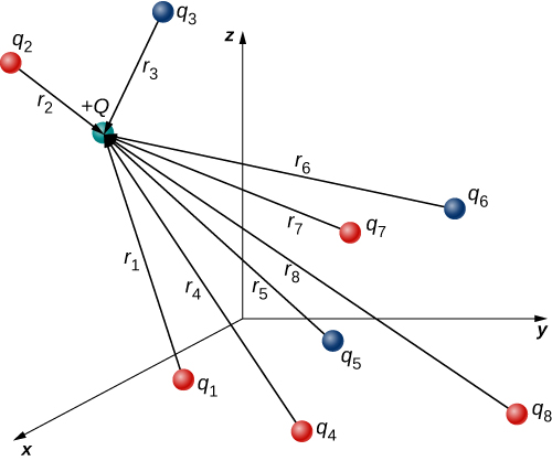
(Note that the force vector $\vec{F}_i$ does not necessarily point in the same direction as the unit vector $\hat{r}_i$; it may point in the opposite direction, $-\hat{r}_i$. The signs of the source charge and test charge determine the direction of the force on the test charge.)

There is a complication, however. Just as the source charges each exert a force on the test charge, so too (by Newton’s third law) does the test charge exert an equal and opposite force on each of the source charges. As a consequence, each source charge would change position. However, by Equation $\ref{Coulomb}$, the force on the test charge is a function of position; thus, as the positions of the source charges change, the net force on the test charge necessarily changes, which changes the force, which again changes the positions. Thus, the entire mathematical analysis quickly becomes intractable. Later, we will learn techniques for handling this situation, but for now, we make the simplifying assumption that the source charges are fixed in place somehow, so that their positions are constant in time. (The test charge is allowed to move.) With this restriction in place, the analysis of charges is known as electrostatics, where “statics” refers to the constant (that is, static) positions of the source charges and the force is referred to as an electrostatic force.

Examples 

Example $\PageIndex{2}$: The Net Force from Two Source Charges

Three different, small charged objects are placed as shown in Figure $\PageIndex{2}$. The charges $q_1$ and $q_3$ are fixed in place; $q_2$ is free to move. Given $q_1 = 2e, \, q_2 = -3e$, and $q_3 = -5e$, and that $d = 2.0 \times 10^{-7} m$, what is the net force on the middle charge $q_2$?

Figure $\PageIndex{4}$: Source charges $q_1$ and $q_3$ each apply a force on $q_2$.

Strategy

We use Coulomb’s law again. The way the question is phrased indicates that $q_2$ is our test charge, so that $q_1$ and $q_3$ are source charges. The principle of superposition says that the force on $q_2$ from each of the other charges is unaffected by the presence of the other charge. Therefore, we write down the force on $q_2$ from each and add them together as vectors.

Solution

We have two source charges $q_1$ and $q_3$ a test charge $q_2$, distances $r_{21}$ and $r_{23}$ and we are asked to find a force. This calls for Coulomb’s law and superposition of forces. There are two forces:

$$\begin{align*} \vec{F}_2 &= \vec{F}_{12} + \vec{F}_{32} = \dfrac{1}{4\pi \epsilon_0}\left[\left(-\dfrac{q_2q_1}{r_{12}^2}\hat{j}\right) + \left(-\dfrac{q_2q_3}{r_{32}^2}\hat{i}\right)\right]. \end{align*}$$

We cannot add these forces directly because they don’t point in the same direction: $\vec{F}_{12}$ points only in the +y-direction, while $\vec{F}_{32}$ points only in the -x-direction. The net force is obtained from applying the Pythagorean theorem to its x- and y-components:

$$F_2 = \sqrt{F_{2x}^2 + F_{2y}^2} \nonumber$$

Thus:

$$\begin{align*} \vec{F}_2 &=  \dfrac{1}{4\pi \epsilon_0}\left[\left(-\dfrac{q_2q_3}{r_{32}^2}\hat{i}\right)+\left(-\dfrac{q_2q_1}{r_{12}^2}\hat{j}\right)\right]. \end{align*}$$

$$\begin{align*} \vec{F}_2 &=  \left(8.99 \times 10^9 \dfrac{N\cdot m^2}{C^2}\right)\left[\left(-\dfrac{(-4.806 \times 10^{-19} C)(-8.01 \times 10^{-19}C)}{(4.00 \times 10^{-7}m)^2}\hat{i}\right)+\left(-\dfrac{(-4.806 \times 10^{-19}C)(3.204 \times 10^{-19}C)}{(2.00 \times 10^{-7} m)^2}\hat{j}\right)\right].\\[4pt] &= - \left(2.16 \times 10^{-14} \, N\right)\hat{i} + \left(3.46 \times 10^{-14} \, N\right)\hat{j}. \end{align*}$$

We find that

$$\begin{align*} F_2 &= \sqrt{F_{2x}^2 + F_{2y}^2} \\[4pt] &= 4.08 \times 10^{-14} \, \text{N} \end{align*}$$

at an angle of

$$\begin{align*} \phi &= \tan^{-1} \left(\dfrac{F_{2y}}{F_{2x}}\right) \\[4pt] &= \tan^{-1} \left( \dfrac{3.46 \times 10^{-14} \text{N}}{-2.16 \times 10^{-14} \text{N}} \right) \\[4pt] &= -58^o, \end{align*}$$

that is, $58^o$ above the −x-axis, as shown in the diagram.

 

Example $\PageIndex{3}$: The Net Force from Three Charges

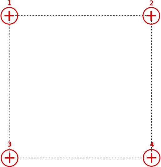
Shown below are 4 identical positive charges located at the corners of a square. The magnitude of the force on charge 1 by charge 4 is $4.0\;\text{N}$.  Find the magnitude of the total force on charge 3 exerted by charges 1, 2, and 4. 

Solution

Let the side of the square be distance a. The relevant distances and forces on charge 3 are shown below.

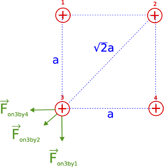
Since the magnitude of the force on charge 1 by charge 4 is 4 N, the same as the magnitude on charge 3 by charge 2 is also 4 N, since the distance between 1 and 4 is the same as between 2 and 3, and the charges are identical, all positive with the same charge $q$. Thus, the magnitude of the force on 3 by 2 is given by:

$$|\vec F_{\text{on 3 by 2}}|=\dfrac{kq}{2a^2}=4 \text{N}\nonumber$$  

The magnitude of the force on 2 by both 1 and 4 are the same since the distance is the same:

$$|\vec F_{\text{on 3 by 1}}|=|\vec F_{\text{on 3 by 4}}|=\dfrac{kq}{a^2}\nonumber$$

Comparing the two equations above we see that the force by 1 and 4 is double the force by 2. Therefore:

$$|\vec F_{\text{on 3 by 1}}|=|\vec F_{\text{on 3 by 4}}|=8 \text{N}\nonumber$$

The direction of the force by 1 is down since the forces are repulsive. In vector form this is written as:

$$\vec F_{\text{on 3 by 1}}=(0,-8) \text{N}\nonumber$$

The direction of the force by 4 is to the left:

$$\vec F_{\text{on 3 by 4}}=(-8,0) \text{N}\nonumber$$

These two vectors combined are:

$$\vec F_{\text{on 3 by 1}}+\vec F_{\text{on 3 by 4}}=(-8,-8) \text{N}\nonumber$$

One way to continue is to break down $\vec F_{\text{on 3 by 2}}$ into components, then add to the sum of the two other forces above, and then find the magnitude. But there is a convenient shortcut when we recognize that the combined vector above will point in the same direction as $\vec F_{\text{on 3 by 2}}$, thus you can just add their magnitudes (it's now a 1D vector addition) to get the total magnitude of the force:

$$|\vec F_{net}|=\sqrt{8^2+8^2}+4=15.3 \text{N}$$

Force Due to a Continuous Charge Distribution

The charge distributions we have seen so far have been discrete: made up of individual point particles. This is in contrast with a continuous charge distribution, which has at least one nonzero dimension. If a charge distribution is continuous rather than discrete, we can generalize the definition of the electric field. We simply divide the charge into infinitesimal pieces and treat each piece as a point charge.

Note that because charge is quantized, there is no such thing as a “truly” continuous charge distribution. However, in most practical cases, the total charge creating the field involves such a huge number of discrete charges that we can safely ignore the discrete nature of the charge and consider it to be continuous. This is exactly the kind of approximation we make when we deal with a bucket of water as a continuous fluid, rather than a collection of $\ce{H2O}$ molecules.

Our first step is to define a charge density for a charge distribution along a line, across a surface, or within a volume, as shown in Figure $\PageIndex{1}$.

Figure $\PageIndex{5}$: The configuration of charge differential elements for a (a) line charge, (b) sheet of charge, and (c) a volume of charge. Also note that (d) some of the components of the total electric field cancel out, with the remainder resulting in a net electric field.

Definitions: Charge Densities

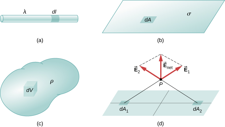
Definitions of charge density:

• linear charge density: $\lambda \equiv$ charge per unit length (Figure $\PageIndex{5a}$); units are coulombs per meter ($C/m$)
• surface charge density: $\sigma \equiv$ charge per unit area (Figure $\PageIndex{5b}$); units are coulombs per square meter $(C/m^2)$
• volume charge density: $\rho \equiv$ charge per unit volume (Figure $\PageIndex{5c}$); units are coulombs per square meter $(C/m^3)$

For a line charge, a surface charge, and a volume charge, the summation in the definition of an Electric field discussed previously becomes an integral and $q_i$ is replaced by $dq = \lambda dl$, $\sigma dA$, or $\rho dV$, respectively:

 

Example $\PageIndex{4}$: Electric Force due to a Ring of Charge

A point charge $q$ is placed a distance $z$ above the center of a ring that has a uniform charge density $\lambda$, with units of coulomb per unit meter of arc, resulting in a total charge of $Q$. Find the electric force acting on the charge $q$.

Strategy

We use the same procedure as for multiple charges. The difference here is that the multiple charges is a charge that is distributed on a circle. We divide the circle into infinitesimal elements shaped as arcs on the circle each having a charge $dq$ and use polar coordinates shown in Figure $\PageIndex{4}$.

Figure $\PageIndex{4}$: The system and variable for calculating the electric force due to a ring of charge.

Solution

The electric force on $q$ due to an arc line charge $dq$ is given by Coulomb's Law:

$$d\vec{F}_q = \dfrac{1}{4\pi \epsilon_0}  \dfrac{dq \ q}{r^2} \hat{r}. \nonumber$$

The charge $dq$ in the arc line charge $dl$ spanning the angle $d\theta$ is given by:

$$dq = \lambda\ dl = \lambda\ (R\ d\theta) . \nonumber$$

The force is then given by:

$$d\vec{F}_q = \dfrac{1}{4\pi \epsilon_0}  \dfrac{\lambda\ R \ d\theta \ q}{r^2} \hat{r}. \nonumber$$

The force due to the whole ring can be obtained through integration:

$$\vec{F}_q = \dfrac{1}{4\pi \epsilon_0} \int_{line} \dfrac{\lambda\ R \ d\theta \ q}{r^2} \hat{r}. \nonumber$$

A general element of the arc between $\theta$ and $\theta + d\theta$ is of length $Rd\theta$ and therefore contains a charge equal to $\lambda R \,d\theta$. The element is at a distance of $r = \sqrt{z^2 + R^2}$ from $P$, the angle is $\cos \, \phi = \dfrac{z}{\sqrt{z^2+R^2}}$ and therefore the electric field is

$$\begin{align*} \vec{E}(P) &= \dfrac{1}{4\pi \epsilon_0} \int_{line} \dfrac{\lambda dl}{r^2} \hat{r} = \dfrac{1}{4\pi \epsilon_0} \int_0^{2\pi} \dfrac{\lambda Rd\theta}{z^2 + R^2} \dfrac{z}{\sqrt{z^2 + R^2}} \hat{z} \\[4pt] &= \dfrac{1}{4\pi \epsilon_0} \dfrac{\lambda Rz}{(z^2 + R^2)^{3/2}} \hat{z} \int_0^{2\pi} d\theta \\[4pt] &= \dfrac{1}{4\pi \epsilon_0} \dfrac{2\pi \lambda Rz}{(z^2 + R^2)^{3/2}} \hat{z} \\[4pt] &= \dfrac{1}{4\pi \epsilon_0} \dfrac{q_{tot}z}{(z^2 + R^2)^{3/2}} \hat{z}. \end{align*}$$

Significance

As usual, symmetry simplified this problem, in this particular case resulting in a trivial integral. Also, when we take the limit of $z \gg R$, we find that

$$\vec{E} \approx \dfrac{1}{4\pi \epsilon_0} \dfrac{q_{tot}}{z^2} \hat{z}, \nonumber$$

as we expect.

Example $\PageIndex{5}$: Electric Force due to a Line Segment along the axis of the segment

Find the electric force on a charge $q$ placed at the origin (point $P$), a distance $a$ to the left of a straight line segment of length $L=b-a$ that carries a uniform positive line charge density $\lambda$ and overall charge $Q$.

Figure $\PageIndex{5}$: A uniformly charged segment of wire. Symmetry implies that the electric field at point $P$ is along the x-axis.

Strategy

Since this is a continuous charge distribution, we conceptually break the wire segment into differential pieces of length $dl$, each of which carries a differential amount of charge

$$dq = \lambda \, dl. \nonumber$$

Then, we conclude that because of symmetry, the force due to each segment is along the x-axis and directed either towards $(-\hat{i})$ or $(+\hat{i})$  depending on the signs of the charges $q$ and $Q$. We then integrate the differential force expression over the length of the wire, from $x = a$ to $x = b$ to obtain the complete electric force expression.

Figure $\PageIndex{4}$: A uniformly charged segment of wire. The electric Force on charge $q$ can be found by applying the superposition principle to charge elements and integrating.

Solution

The electric force due to a line charge segment  $dl$ on the charge  $q$ is given by the general Coulomb expression:

$$d\vec{F}_q = \dfrac{1}{4\pi \epsilon_0} \dfrac{(\lambda\ dl)\ q}{r^2}\hat{i}. \nonumber$$

The electric force due to the whole line charge segment  on the charge  $q$ can be found through integration over the whole line segment:

$$\vec{F}_q = \dfrac{1}{4\pi \epsilon_0} \int_{line} \dfrac{(\lambda\ dl)\ q}{r^2}\hat{i}. \nonumber$$

The symmetry of the situation implies that there are only horizontal ($x$)-components of the Force. The drawing implies that the charges are identical in sign resulting in a repulsive force. However, the calculation will maintain the vector notation to ensure that the final expression will work for whatever charge sign configuration. 

So we have

$$\begin{align*}\vec{F}_q &= \dfrac{-1}{4 \pi \epsilon_0}\int \dfrac{(\lambda dl)\ q}{r^2} \, \hat{i} \\[4pt] &= \dfrac{-1}{4 \pi \epsilon_0}\int_{a}^{b} \dfrac{(\lambda dx)\ q}{x^2} \, \hat{i} \end{align*}$$

where our differential line element $dl$ is $dx$, in this example, since we are integrating along a line of charge that lies on the $x$-axis. (The limits of integration are $a$ to $b$.

$$\begin{align*} \vec{F}_q &= \dfrac{1}{4 \pi \epsilon_0}\int_{a}^{b} \dfrac{(\lambda dx)\ q}{x^2} \, \hat{i}\\[4pt] &= \dfrac{\lambda \ q}{4 \pi \epsilon_0} \left[\dfrac{1}{x}\right]_{a}^{b} \, \hat{i}\\[4pt] &= \dfrac{\lambda \ q}{4 \pi \epsilon_0} \left[\dfrac{-1}{b} - \dfrac{-1}{a}\right] \, \hat{i}\\[4pt] &= \dfrac{\lambda \ q}{4 \pi \epsilon_0} \left[\dfrac{1}{a} - \dfrac{1}{b}\right] \, \hat{i}. \end{align*}\nonumber$$

The result is then:

$$\vec{F}_q = \dfrac{\lambda \ q}{4 \pi \epsilon_0} \left( \dfrac{1}{a} -  \dfrac{1}{b} \right)\, \hat{i}. \nonumber$$