Plot ordered pairs in a Cartesian coordinate system.
Graph equations by plotting points.
Graph equations with a graphing utility.
Find \(x\)-intercepts and \(y\)-intercepts.
Use the distance formula.
Use the midpoint formula.
Plotting Ordered Pairs in the Cartesian Coordinate System
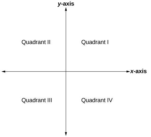
The Cartesian coordinate system, also called the rectangular coordinate system, is based on a two-dimensional plane consisting of the \(x\)-axis and the \(y\)-axis. Perpendicular to each other, the axes divide the plane into four sections. Each section is called a quadrant; the quadrants are numbered counterclockwise as shown in Figure \(\PageIndex{2}\).
Figure \(\PageIndex{2}\)
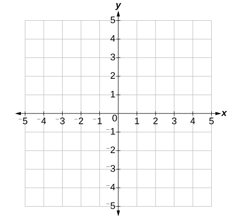
The center of the plane is the point at which the two axes cross. It is known as the origin, or point \((0,0)\). From the origin, each axis is further divided into equal units: increasing, positive numbers to the right on the \(x\)-axis and up the \(y\)-axis; decreasing, negative numbers to the left on the \(x\)-axis and down the \(y\)-axis. The axes extend to positive and negative infinity as shown by the arrowheads in Figure \(\PageIndex{3}\).
Figure \(\PageIndex{3}\)
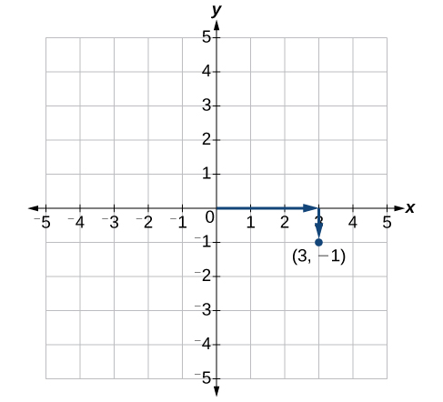
Each point in the plane is identified by its \(x\)-coordinate, or horizontal displacement from the origin, and its \(y\)-coordinate, or vertical displacement from the origin. Together, we write them as an ordered pair indicating the combined distance from the origin in the form \((x,y)\). An ordered pair is also known as a coordinate pair because it consists of \(x\)- and \(y\)-coordinates. For example, we can represent the point \((3,−1)\) in the plane by moving three units to the right of the origin in the horizontal direction, and one unit down in the vertical direction. See Figure \(\PageIndex{4}\).
Figure \(\PageIndex{4}\)
When dividing the axes into equally spaced increments, note that the \(x\)-axis may be considered separately from the \(y\)-axis. In other words, while the \(x\)-axis may be divided and labeled according to consecutive integers, the \(y\)-axis may be divided and labeled by increments of \(2\), or \(10\), or \(100\). In fact, the axes may represent other units, such as years against the balance in a savings account, or quantity against cost, and so on. Consider the rectangular coordinate system primarily as a method for showing the relationship between two quantities.
Cartesian Coordinate System
A two-dimensional plane where the
\(x\)-axis is the horizontal axis
\(y\)-axis is the vertical axis
A point in the plane is defined as an ordered pair, \((x,y)\), such that \(x\) is determined by its horizontal distance from the origin and \(y\) is determined by its vertical distance from the origin.
Example \(\PageIndex{1}\): Plotting Points in a Rectangular Coordinate System
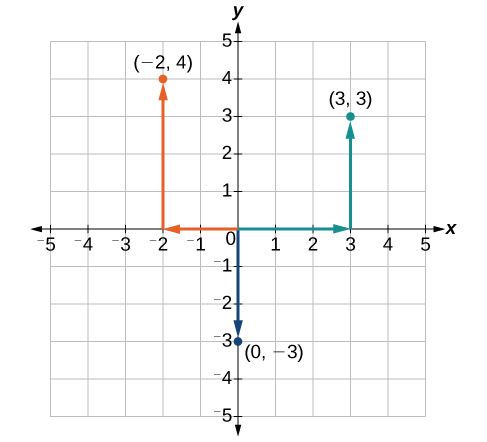
Plot the points \((−2,4)\), \((3,3)\), and \((0,−3)\) in the plane.
Solution
To plot the point \((−2,4)\), begin at the origin. The \(x\)-coordinate is \(–2\), so move two units to the left. The \(y\)-coordinate is \(4\), so then move four units up in the positive \(y\) direction.
To plot the point \((3,3)\), begin again at the origin. The \(x\)-coordinate is \(3\), so move three units to the right. The \(y\)-coordinate is also \(3\), so move three units up in the positive \(y\) direction.
To plot the point \((0,−3)\), begin again at the origin. The \(x\)-coordinate is \(0\). This tells us not to move in either direction along the \(x\)-axis. The \(y\)-coordinate is \(–3\), so move three units down in the negative \(y\) direction. See the graph in Figure \(\PageIndex{5}\).
Figure \(\PageIndex{5}\)Analysis
Note that when either coordinate is zero, the point must be on an axis. If the \(x\)-coordinate is zero, the point is on the \(y\)-axis. If the \(y\)-coordinate is zero, the point is on the \(x\)-axis.
Graphing Equations by Plotting Points
We can plot a set of points to represent an equation. When such an equation contains both an \(x\) variable and a \(y\) variable, it is called an equation in two variables. Its graph is called a graph in two variables. Any graph on a two-dimensional plane is a graph in two variables.
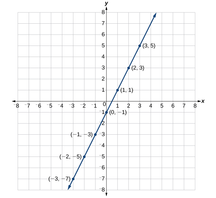
Suppose we want to graph the equation \(y=2x−1\). We can begin by substituting a value for \(x\) into the equation and determining the resulting value of \(y\). Each pair of \(x\)- and \(y\)-values is an ordered pair that can be plotted. Table \(\PageIndex{1}\) lists values of \(x\) from \(–3\) to \(3\) and the resulting values for \(y\).
Table \(\PageIndex{1}\)
\(x\)
\(y=2x−1\)
\((x,y)\)
\(−3\)
\(y=2(−3)−1=−7\)
\((−3,−7)\)
\(−2\)
\(y=2(−2)−1=−5\)
\((−2,−5)\)
\(−1\)
\(y=2(−1)−1=−3\)
\((−1,−3)\)
\(0\)
\(y=2(0)−1=−1\)
\((0,−1)\)
\(1\)
\(y=2(1)−1=1\)
\((1,1)\)
\(2\)
\(y=2(2)−1=3\)
\((2,3)\)
\(3\)
\(y=2(3)−1=5\)
\((3,5)\)
We can plot the points in the table. The points for this particular equation form a line, so we can connect them (Figure \(\PageIndex{6}\)). This is not true for all equations.
Figure \(\PageIndex{6}\)
Note that the \(x\)-values chosen are arbitrary, regardless of the type of equation we are graphing. Of course, some situations may require particular values of \(x\) to be plotted in order to see a particular result. Otherwise, it is logical to choose values that can be calculated easily, and it is always a good idea to choose values that are both negative and positive. There is no rule dictating how many points to plot, although we need at least two to graph a line. Keep in mind, however, that the more points we plot, the more accurately we can sketch the graph.
Howto: Given an equation, graph by plotting points
Make a table with one column labeled \(x\), a second column labeled with the equation, and a third column listing the resulting ordered pairs.
Enter \(x\)-values down the first column using positive and negative values. Selecting the \(x\)-values in numerical order will make the graphing simpler.
Select \(x\)-values that will yield \(y\)-values with little effort, preferably ones that can be calculated mentally.
Plot the ordered pairs.
Connect the points if they form a line.
Example \(\PageIndex{2}\): Graphing an Equation in Two Variables by Plotting Points
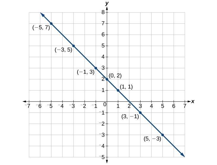
Graph the equation \(y=−x+2\) by plotting points.
Solution
First, we construct a table similar to Table \(\PageIndex{2}\). Choose \(x\) values and calculate \(y\).
Table \(\PageIndex{2}\)
\(x\)
\(y=−x+2\)
\((x,y)\)
\(−5\)
\(y=−(−5)+2=7\)
\((−5,7)\)
\(−3\)
\(y=−(−3)+2=5\)
\((−3,5)\)
\(−1\)
\(y=−(−1)+2=3\)
\((−1,3)\)
\(0\)
\(y=−(0)+2=2\)
\((0,2)\)
\(1\)
\(y=−(1)+2=1\)
\((1,1)\)
\(3\)
\(y=−(3)+2=−1\)
\((3,−1)\)
\(5\)
\(y=−(5)+2=−3\)
\((5,−3)\)
Now, plot the points. Connect them if they form a line. See Figure \(\PageIndex{7}\).
Figure \(\PageIndex{7}\)
Finding \(x\)-intercepts and \(y\)-intercepts
The intercepts of a graph are points at which the graph crosses the axes. The \(x\)-intercept is the point at which the graph crosses the \(x\)-axis. At this point, the \(y\)-coordinate is zero. The \(y\)-intercept is the point at which the graph crosses the \(y\)-axis. At this point, the \(x\)-coordinate is zero.
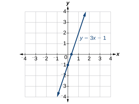
To determine the \(x\)-intercept, we set \(y\) equal to zero and solve for \(x\). Similarly, to determine the \(y\)-intercept, we set \(x\) equal to zero and solve for \(y\). For example, lets find the intercepts of the equation \(y=3x−1\).
To find the \(x\)-intercept, set \(y=0\).
\[\begin{align*} y &= 3x - 1\\ 0 &= 3x - 1\\ 1 &= 3x\\ \dfrac{1}{3}&= x \end{align*}\]
\(x\)−intercept:\(\left(\dfrac{1}{3},0\right)\)
To find the \(y\)-intercept, set \(x=0\).
\[\begin{align*} y &= 3x - 1\\ y &= 3(0) - 1\\ y &= -1 \end{align*}\]
\(y\)−intercept:\((0,−1)\)
We can confirm that our results make sense by observing a graph of the equation as in Figure \(\PageIndex{12}\). Notice that the graph crosses the axes where we predicted it would.
Figure \(\PageIndex{12}\)
Howto: GIVEN AN EQUATION, FIND THE INTERCEPTS
Find the \(x\)-intercept by setting \(y=0\) and solving for \(x\).
Find the \(y\)-intercept by setting \(x=0\) and solving for \(y\).
Example \(\PageIndex{3}\): Finding the Intercepts of the Given Equation
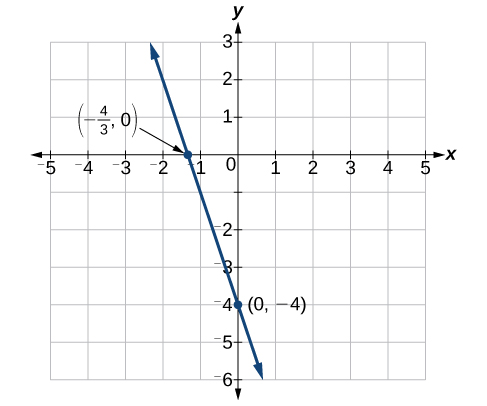
Find the intercepts of the equation \(y=−3x−4\). Then sketch the graph using only the intercepts.
Solution
Set \(y=0\) to find the \(x\)-intercept.
\[\begin{align*} y &= -3x - 4\\ 0 &= -3x - 4\\ 4 &= -3x\\ \dfrac{4}{3}&= x \end{align*}\]
\(x\)−intercept:\(\left(−\dfrac{4}{3},0\right)\)
Set \(x=0\) to find the \(y\)-intercept.
\[\begin{align*} y &= -3x - 4\\ y &= -3(0) - 4\\ y &= -4 \end{align*}\]
\(y\)−intercept: \((0,−4)\)
Plot both points, and draw a line passing through them as in Figure \(\PageIndex{13}\).
Figure \(\PageIndex{13}\)
Using the Distance Formula
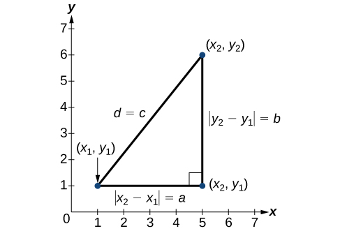
Derived from the Pythagorean Theorem, the distance formula is used to find the distance between two points in the plane. The Pythagorean Theorem, \(a^2+b^2=c^2\), is based on a right triangle where \(a\) and \(b\) are the lengths of the legs adjacent to the right angle, and \(c\) is the length of the hypotenuse. See Figure \(\PageIndex{15}\).
Figure \(\PageIndex{15}\)
The relationship of sides \(|x_2−x_1|\) and \(|y_2−y_1|\) to side \(d\) is the same as that of sides \(a\) and \(b\) to side \(c\). We use the absolute value symbol to indicate that the length is a positive number because the absolute value of any number is positive. (For example, \(|-3|=3\). ) The symbols \(|x_2−x_1|\) and \(|y_2−y_1|\) indicate that the lengths of the sides of the triangle are positive. To find the length \(c\), take the square root of both sides of the Pythagorean Theorem.
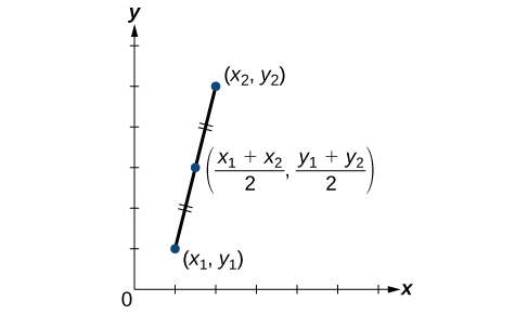
When the endpoints of a line segment are known, we can find the point midway between them. This point is known as the midpoint and the formula is known as the midpoint formula. Given the endpoints of a line segment, \((x_1,y_1)\) and \((x_2,y_2)\), the midpoint formula states how to find the coordinates of the midpoint M.
We can locate, or plot, points in the Cartesian coordinate system using ordered pairs, which are defined as displacement from the \(x\)-axis and displacement from the \(y\)-axis. See Example.
An equation can be graphed in the plane by creating a table of values and plotting points. See Example.
Using a graphing calculator or a computer program makes graphing equations faster and more accurate. Equations usually have to be entered in the form \(y=\)_____. See Example.
Finding the \(x\)- and \(y\)-intercepts can define the graph of a line. These are the points where the graph crosses the axes. See Example.
The distance formula is derived from the Pythagorean Theorem and is used to find the length of a line segment. See Example and Example.
The midpoint formula provides a method of finding the coordinates of the midpoint dividing the sum of the \(x\)-coordinates and the sum of the \(y\)-coordinates of the endpoints by \(2\). See Example and Example.