2.7.11: Functions

Learning Objectives

• Use functional notation to evaluate a function.
• Determine the domain and range of a function.
• Draw the graph of a function.
• Find the zeros of a function.
• Make new functions from two or more given functions.
• Describe the symmetry properties of a function.
• Determine the conditions for when a function has an inverse.
• Use the horizontal line test to recognize when a function is one-to-one.
• Find the inverse of a given function.
• Draw the graph of an inverse function.

Functions

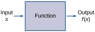
Given two sets \(A\) and \(B\) a set with elements that are ordered pairs \((x,y)\) where \(x\) is an element of \(A\) and \(y\) is an element of \(B,\) is a relation from \(A\) to \(B\). A relation from \(A\) to \(B\) defines a relationship between those two sets. A function is a special type of relation in which each element of the first set is related to exactly one element of the second set. The element of the first set is called the input; the element of the second set is called the output. Functions are used all the time in mathematics to describe relationships between two sets. For any function, when we know the input, the output is determined, so we say that the output is a function of the input. For example, the area of a square is determined by its side length, so we say that the area (the output) is a function of its side length (the input). The velocity of a ball thrown in the air can be described as a function of the amount of time the ball is in the air. The cost of mailing a package is a function of the weight of the package. Since functions have so many uses, it is important to have precise definitions and terminology to study them.

Figure \(\PageIndex{1}\): A function can be visualized as an input/output device

Definition: Functions

A function \(f\) consists of a set of inputs, a set of outputs, and a rule for assigning each input to exactly one output. The set of inputs is called the domain of the function. The set of outputs is called the range of the function.

Figure \(\PageIndex{2}\): A function maps every element in the domain to exactly one element in the range. Although each input can be sent to only one output, two different inputs can be sent to the same output.

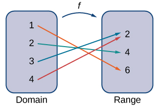
For example, consider the function \(f\), where the domain is the set of all real numbers and the rule is to square the input. Then, the input \(x=3\) is assigned to the output \(3^2=9\).

Since every nonnegative real number has a real-value square root, every nonnegative number is an element of the range of this function. Since there is no real number with a square that is negative, the negative real numbers are not elements of the range. We conclude that the range is the set of nonnegative real numbers.

For a general function \(f\) with domain \(D\), we often use \(x\) to denote the input and \(y\) to denote the output associated with \(x\). When doing so, we refer to \(x\) as the independent variable and \(y\) as the dependent variable, because it depends on \(x\). Using function notation, we write \(y=f(x)\), and we read this equation as “\(y\) equals \(f\) of \(x.”\) For the squaring function described earlier, we write \(f(x)=x^2\).

Algebraic Formulas

Sometimes we are given a function in an explicit formula. Formulas arise in many applications. For example, the area of a circle of radius \(r\) is given by the formula \(A(r)=πr^2\). When an object is thrown upward from the ground with an initial velocity \(v_{0}\) ft/s, its height above the ground from the time it is thrown until it hits the ground is given by the formula \(s(t)=−16t^2+v_{0}t\). When \(P\) dollars are invested in an account at an annual interest rate \(r\) compounded continuously, the amount of money after \(t\) years is given by the formula \(A(t)=Pe^{rt}\). Algebraic formulas are important tools to calculate function values. Often we also represent these functions visually in graph form.

Given an algebraic formula for a function \(f\), the graph of \(f\) is the set of points \((x,f(x))\), where \(x\) is in the domain of \(f\) and \(f(x)\) is in the range. To graph a function given by a formula, it is helpful to begin by using the formula to create a table of inputs and outputs. If the domain of \(f\) consists of an infinite number of values, we cannot list all of them, but because listing some of the inputs and outputs can be very useful, it is often a good way to begin.

When creating a table of inputs and outputs, we typically check to determine whether zero is an output. Those values of \(x\) where \(f(x)=0\) are called the zeros of a function. For example, the zeros of \(f(x)=x^2−4\) are \(x=±2\). The zeros determine where the graph of \(f\) intersects the \(x\)-axis, which gives us more information about the shape of the graph of the function. The graph of a function may never intersect the \(x\)-axis, or it may intersect multiple (or even infinitely many) times.

Another point of interest is the \(y\) -intercept, if it exists. The \(y\)-intercept is given by \((0,f(0))\).

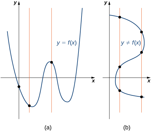
Since a function has exactly one output for each input, the graph of a function can have, at most, one \(y\)-intercept. If \(x=0\) is in the domain of a function \(f,\) then \(f\) has exactly one \(y\)-intercept. If \(x=0\) is not in the domain of \(f,\) then \(f\) has no \(y\)-intercept. Similarly, for any real number \(c,\) if \(c\) is in the domain of \(f\), there is exactly one output \(f(c),\) and the line \(x=c\) intersects the graph of \(f\) exactly once. On the other hand, if \(c\) is not in the domain of \(f,\) \(f(c)\) is not defined and the line \(x=c\) does not intersect the graph of \(f\). This property is summarized in the vertical line test.

Vertical Line Test

Given a function \(f\), every vertical line that may be drawn intersects the graph of \(f\) no more than once. If any vertical line intersects a set of points more than once, the set of points does not represent a function.

We can use this test to determine whether a set of plotted points represents the graph of a function (Figure \(\PageIndex{7}\)).

Figure \(\PageIndex{7}\): (a) The set of plotted points represents the graph of a function because every vertical line intersects the set of points, at most, once. (b) The set of plotted points does not represent the graph of a function because some vertical lines intersect the set of points more than once.

Example \(\PageIndex{3}\): Finding Zeros and \(y\)-Intercepts of a Function

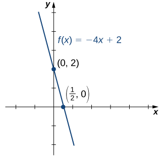
Consider the function \(f(x)=−4x+2.\)

1. Find all zeros of \(f\).
2. Find the \(y\)-intercept (if any).
3. Sketch a graph of \(f\).

Solution

1.To find the zeros, solve \(f(x)=−4x+2=0\). We discover that \(f\) has one zero at \(x=1/2\).

2. The \(y\)-intercept is given by \((0,f(0))=(0,2).\)

3. Given that \(f\) is a linear function of the form \(f(x)=mx+b\) that passes through the points \((1/2,0)\) and \((0,2)\), we can sketch the graph of \(f\) (Figure \(\PageIndex{8}\)).

Figure \(\PageIndex{8}\): The function \(f(x)=−4x+2\) is a line with \(x\)-intercept \((1/2,0)\) and \(y\)-intercept \((0,2)\).

Example \(\PageIndex{4}\): Using Zeros and \(y\)-Intercepts to Sketch a Graph

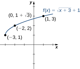
Consider the function \(f(x)=\sqrt{x+3}+1\).

1. Find all zeros of \(f\).
2. Find the \(y\)-intercept (if any).
3. Sketch a graph of \(f\).

Solution

1.To find the zeros, solve \(\sqrt{x+3}+1=0\). This equation implies \(\sqrt{x+3}=−1\). Since \(\sqrt{x+3}≥0\) for all \(x\), this equation has no solutions, and therefore \(f\) has no zeros.

2.The \(y\)-intercept is given by \((0,f(0))=(0,\sqrt{3}+1)\).

3.To graph this function, we make a table of values. Since we need \(x+3≥0\), we need to choose values of \(x≥−3\). We choose values that make the square-root function easy to evaluate.

\(x\)	-3	-2	1
\(f(x)\)	1	2	3

Making use of the table and knowing that, since the function is a square root, the graph of \(f\) should be similar to the graph of \(y=\sqrt{x}\), we sketch the graph (Figure \(\PageIndex{9}\)).

Figure \(\PageIndex{9}\): The graph of \(f(x)=\sqrt{x+3}+1\) has a \(y\)-intercept but no \(x\)-intercepts.

Exercise \(\PageIndex{4}\)

Find the zeros of \(f(x)=x^3−5x^2+6x.\)

Hint

Factor the polynomial.

Answer

\(x=0,2,3\)

Example \(\PageIndex{5}\): Finding the Height of a Free-Falling Object

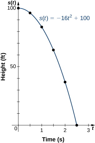
If a ball is dropped from a height of 100 ft, its height s at time \(t\) is given by the function \(s(t)=−16t^2+100\), where s is measured in feet and \(t\) is measured in seconds. The domain is restricted to the interval \([0,c],\) where \(t=0\) is the time when the ball is dropped and \(t=c\) is the time when the ball hits the ground.

1. Create a table showing the height s(t) when \(t=0,\, 0.5,\, 1,\, 1.5,\, 2,\) and \(2.5\). Using the data from the table, determine the domain for this function. That is, find the time \(c\) when the ball hits the ground.
2. Sketch a graph of \(s\).

Solution

\(t\)	0	0.5	1	1.5	2	2.5
\(s(t)\)	100	96	84	64	36	0

Since the ball hits the ground when \(t=2.5\), the domain of this function is the interval \([0,2.5]\).

2.

Figure \(\PageIndex{8}\), the values of \(f(x)\) are getting smaller as \(x\) is getting larger. A function with this property is said to be decreasing. On the other hand, for the function \(f(x)=\sqrt{x+3}+1\) graphed in Figure \(\PageIndex{9}\), the values of \(f(x)\) are getting larger as the values of \(x\) are getting larger. A function with this property is said to be increasing. It is important to note, however, that a function can be increasing on some interval or intervals and decreasing over a different interval or intervals. For example, using our temperature function plotted above, we can see that the function is decreasing on the interval \((0,4)\), increasing on the interval \((4,14)\), and then decreasing on the interval \((14,23)\). We make the idea of a function increasing or decreasing over a particular interval more precise in the next definition.

Definition: Increasing and Decreasing on an Interval

We say that a function \(f\) is increasing on the interval \(I\) if for all \(x_{1},\, x_{2}∈I,\)

\(f(x_{1})≤f(x_{2})\) when \(x_{1}<x_{2}.\)

We say \(f\) is strictly increasing on the interval \(I\) if for all \(x_{1},x_{2}∈I,\)

\(f(x_{1})<f(x_{2})\) when \(x_{1}<x_{2}.\)

We say that a function \(f\) is decreasing on the interval \(I\) if for all \(x_{1},x_{2}∈I,\)

\(f(x_{1})≥f(x_{2})\) if \(x_{1}<x_{2}.\)

We say that a function \(f\) is strictly decreasing on the interval \(I\) if for all \(x_{1},x_{2}∈I\),

\(f(x_{1})>f(x_{2})\) if \(x_{1}<x_{2}.\)

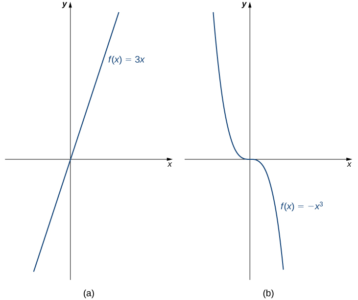
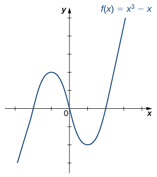
For example, the function \(f(x)=3x\) is increasing on the interval \((−∞,∞)\) because \(3x_{1}<3x_{2}\) whenever \(x_{1}<x_{2}\). On the other hand, the function \(f(x)=−x^3\) is decreasing on the interval \((−∞,∞)\) because \(−x^3_{1}>−x^3_{2}\) whenever \(x_{1}<x_{2}\) (Figure \(\PageIndex{10}\)).

Figure \(\PageIndex{10}\): (a) The function \(f(x)=3x\) is increasing on the interval \((−∞,∞)\). (b) The function \(f(x)=−x^3\) is decreasing on the interval \((−∞,∞)\).

Combining Functions

Now that we have reviewed the basic characteristics of functions, we can see what happens to these properties when we combine functions in different ways, using basic mathematical operations to create new functions. For example, if the cost for a company to manufacture \(x\) items is described by the function \(C(x)\) and the revenue created by the sale of \(x\) items is described by the function \(R(x)\), then the profit on the manufacture and sale of \(x\) items is defined as \(P(x)=R(x)−C(x)\). Using the difference between two functions, we created a new function.

Alternatively, we can create a new function by composing two functions. For example, given the functions \(f(x)=x^2\) and \(g(x)=3x+1\), the composite function \(f∘g\) is defined such that

\[(f∘g)(x)=f(g(x))=(g(x))^2=(3x+1)^2. \nonumber \]

The composite function \(g∘f\) is defined such that

\[(g∘f)(x)=g(f(x))=3f(x)+1=3x^2+1. \nonumber \]

Note that these two new functions are different from each other.

Combining Functions with Mathematical Operators

To combine functions using mathematical operators, we simply write the functions with the operator and simplify. Given two functions \(f\) and \(g\), we can define four new functions:

\((f+g)(x)=f(x)+g(x)\)	Sum
\((f−g)(x)=f(x)−g(x)\)	Difference
\((f·g)(x)=f(x)g(x)\)	Product
\((\frac{f}{g})(x)=\frac{f(x)}{g(x)}\) for\(g(x)≠0\)	Quotient

Example \(\PageIndex{6}\): Combining Functions Using Mathematical Operations

Given the functions \(f(x)=2x−3\) and \(g(x)=x^2−1\), find each of the following functions and state its domain.

1. \((f+g)(x)\)
2. \((f−g)(x)\)
3. \((f·g)(x)\)
4. \(\left(\dfrac{f}{g}\right)(x)\)

Solution

1. \((f+g)(x)=(2x−3)+(x^2−1)=x^2+2x−4.\)

The domain of this function is the interval \((−∞,∞)\).

2.\((f−g)(x)=(2x−3)−(x^2−1)=−x^2+2x−2.\)

The domain of this function is the interval \((−∞,∞)\).

3. \((f·g)(x)=(2x−3)(x^2−1)=2x^3−3x^2−2x+3.\)

The domain of this function is the interval \((−∞,∞)\).

4. \(\left(\dfrac{f}{g}\right)(x)=\dfrac{2x−3}{x^2−1}\).

The domain of this function is \(\{x\,|\,x≠±1\}.\)

Exercise \(\PageIndex{6}\)

For \(f(x)=x^2+3\) and \(g(x)=2x−5\), find \((f/g)(x)\) and state its domain.

Hint

The new function \((f/g)(x)\) is a quotient of two functions. For what values of \(x\) is the denominator zero?

Answer

\(\left(\dfrac{f}{g}\right)(x)=\frac{x^2+3}{2x−5}.\) The domain is \(\{x\,|\,x≠\frac{5}{2}\}.\)

Function Composition

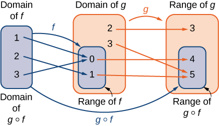
When we compose functions, we take a function of a function. For example, suppose the temperature \(T\) on a given day is described as a function of time \(t\) (measured in hours after midnight) as in Table \(\PageIndex{1}\). Suppose the cost \(C\), to heat or cool a building for 1 hour, can be described as a function of the temperature \(T\). Combining these two functions, we can describe the cost of heating or cooling a building as a function of time by evaluating \(C(T(t))\). We have defined a new function, denoted \(C∘T\), which is defined such that \((C∘T)(t)=C(T(t))\) for all \(t\) in the domain of \(T\). This new function is called a composite function. We note that since cost is a function of temperature and temperature is a function of time, it makes sense to define this new function \((C∘T)(t)\). It does not make sense to consider \((T∘C)(t)\), because temperature is not a function of cost.

Definition: Composite Functions

Consider the function \(f\) with domain \(A\) and range \(B\), and the function \(g\) with domain \(D\) and range \(E\). If \(B\) is a subset of \(D\), then the composite function \((g∘f)(x)\) is the function with domain \(A\) such that

\[(g∘f)(x)=g(f(x)) \nonumber \]

A composite function \(g∘f\) can be viewed in two steps. First, the function \(f\) maps each input \(x\) in the domain of \(f\) to its output \(f(x)\) in the range of \(f\). Second, since the range of \(f\) is a subset of the domain of \(g\), the output \(f(x)\) is an element in the domain of \(g\), and therefore it is mapped to an output \(g(f(x))\) in the range of \(g\). In Figure \(\PageIndex{11}\), we see a visual image of a composite function.

Figure \(\PageIndex{11}\): For the composite function \(g∘f\), we have \((g∘f)(1)=4,\) \((g∘f)(2)=5,\) and \((g∘f)(3)=4\).

Example \(\PageIndex{7}\): Compositions of Functions Defined by Formulas

Consider the functions \(f(x)=x^2+1\) and \(g(x)=1/x\).

1. Find \((g∘f)(x)\) and state its domain and range.
2. Evaluate \((g∘f)(4),\) \((g∘f)(−1/2)\).
3. Find \((f∘g)(x)\) and state its domain and range.
4. Evaluate \((f∘g)(4),\) \((f∘g)(−1/2)\).

Solution

1. We can find the formula for \((g∘f)(x)\) in two different ways. We could write

\((g∘f)(x)=g(f(x))=g(x^2+1)=\dfrac{1}{x^2+1}\).

Alternatively, we could write

\((g∘f)(x)=g(f(x))=\dfrac{1}{f(x)}=\dfrac{1}{x^2+1}.\)

Since \(x^2+1≠0\) for all real numbers \(x,\) the domain of \((g∘f)(x)\) is the set of all real numbers. Since \(0<1/(x^2+1)≤1\), the range is, at most, the interval \((0,1]\). To show that the range is this entire interval, we let \(y=1/(x^2+1)\) and solve this equation for \(x\) to show that for all \(y\) in the interval \((0,1]\), there exists a real number \(x\) such that \(y=1/(x^2+1)\). Solving this equation for \(x,\) we see that \(x^2+1=1/y\), which implies that

\(x=±\sqrt{\frac{1}{y}−1}\)

If \(y\) is in the interval \((0,1]\), the expression under the radical is nonnegative, and therefore there exists a real number \(x\) such that \(1/(x^2+1)=y\). We conclude that the range of \(g∘f\) is the interval \((0,1].\)

2. \((g∘f)(4)=g(f(4))=g(4^2+1)=g(17)=\frac{1}{17}\)

\((g∘f)(−\frac{1}{2})=g(f(−\frac{1}{2}))=g((−\frac{1}{2})^2+1)=g(\frac{5}{4})=\frac{4}{5}\)

3. We can find a formula for \((f∘g)(x)\) in two ways. First, we could write

\((f∘g)(x)=f(g(x))=f(\frac{1}{x})=(\frac{1}{x})^2+1.\)

Alternatively, we could write

\((f∘g)(x)=f(g(x))=(g(x))^2+1=(\frac{1}{x})^2+1.\)

The domain of \(f∘g\) is the set of all real numbers \(x\) such that \(x≠0\). To find the range of \(f,\) we need to find all values \(y\) for which there exists a real number \(x≠0\) such that

\(\left(\dfrac{1}{x}\right)^2+1=y.\)

Solving this equation for \(x,\) we see that we need \(x\) to satisfy

\(\left(\dfrac{1}{x}\right)^2=y−1,\)

which simplifies to

\(\dfrac{1}{x}=±\sqrt{y−1}\)

Finally, we obtain

\(x=±\dfrac{1}{\sqrt{y−1}}.\)

Since \(1/\sqrt{y−1}\) is a real number if and only if \(y>1,\) the range of \(f\) is the set \(\{y\,|\,y≥1\}.\)

4.\((f∘g)(4)=f(g(4))=f(\frac{1}{4})=(\frac{1}{4})^2+1=\frac{17}{16}\)

\((f∘g)(−\frac{1}{2})=f(g(−\frac{1}{2}))=f(−2)=(−2)^2+1=5\)

In Example \(\PageIndex{7}\), we can see that \((f∘g)(x)≠(g∘f)(x)\). This tells us, in general terms, that the order in which we compose functions matters.

Exercise \(\PageIndex{7}\)

Let \(f(x)=2−5x\). Let \(g(x)=\sqrt{x}.\) Find \((f∘g)(x)\).

Solution

\((f∘g)(x)=2−5\sqrt{x}.\)

Symmetry of Functions

The graphs of certain functions have symmetry properties that help us understand the function and the shape of its graph. For example, consider the function \(f(x)=x^4−2x^2−3\) shown in Figure \(\PageIndex{12a}\). If we take the part of the curve that lies to the right of the \(y\)-axis and flip it over the \(y\)-axis, it lays exactly on top of the curve to the left of the \(y\)-axis. In this case, we say the function has symmetry about the \(y\)-axis. On the other hand, consider the function \(f(x)=x^3−4x\) shown in Figure \(\PageIndex{12b}\). If we take the graph and rotate it \(180°\) about the origin, the new graph will look exactly the same. In this case, we say the function has symmetry about the origin.

Figure \(\PageIndex{12}\): (a) A graph that is symmetric about the \(y\)-axis. (b) A graph that is symmetric about the origin.

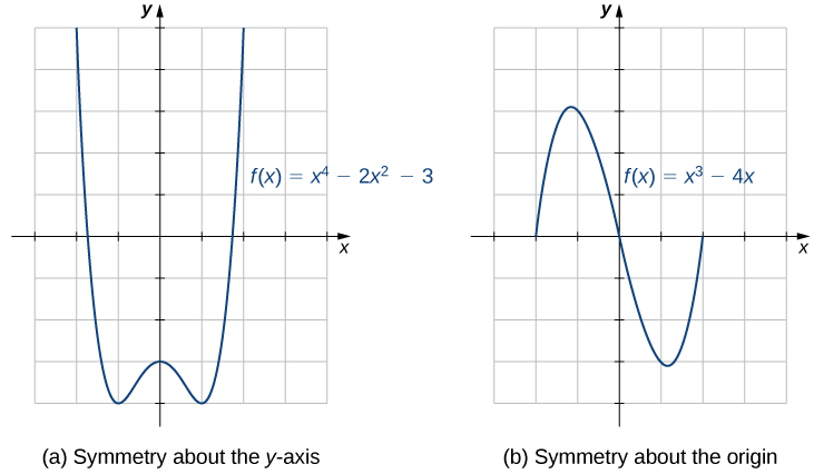
If we are given the graph of a function, it is easy to see whether the graph has one of these symmetry properties. But without a graph, how can we determine algebraically whether a function \(f\) has symmetry? Looking at Figure \(\PageIndex{12a}\) again, we see that since \(f\) is symmetric about the \(y\)-axis, if the point \((x,y)\) is on the graph, the point \((−x,y)\) is on the graph. In other words, \(f(−x)=f(x)\). If a function \(f\) has this property, we say \(f\) is an even function, which has symmetry about the \(y\)-axis. For example, \(f(x)=x^2\) is even because

\(f(−x)=(−x)^2=x^2=f(x).\)

In contrast, looking at Figure \(\PageIndex{12b}\) again, if a function \(f\) is symmetric about the origin, then whenever the point \((x,y)\) is on the graph, the point \((−x,−y)\) is also on the graph. In other words, \(f(−x)=−f(x)\). If \(f\) has this property, we say \(f\) is an odd function, which has symmetry about the origin. For example, \(f(x)=x^3\) is odd because

\(f(−x)=(−x)^3=−x^3=−f(x).\)

Definition: Even and Odd Functions

• If \(f(x)=f(−x)\) for all \(x\) in the domain of \(f\), then \(f\) is an even function. An even function is symmetric about the \(y\)-axis.
• If \(f(−x)=−f(x)\) for all \(x\) in the domain of \(f\), then \(f\) is an odd function. An odd function is symmetric about the origin.

Example \(\PageIndex{10}\): Even and Odd Functions

Determine whether each of the following functions is even, odd, or neither.

1. \(f(x)=−5x^4+7x^2−2\)
2. \(f(x)=2x^5−4x+5\)
3. \(f(x)=\frac{3x}{x^2+1}\)

Solution

To determine whether a function is even or odd, we evaluate \(f(−x)\) and compare it to \(f(x)\) and \(−f(x)\).

1. \(f(−x)=−5(−x)^4+7(−x)^2−2=−5x^4+7x^2−2=f(x).\) Therefore, \(f\) is even.

2.\(f(−x)=2(−x)^5−4(−x)+5=−2x^5+4x+5.\) Now, \(f(−x)≠f(x).\) Furthermore, noting that \(−f(x)=−2x^5+4x−5\), we see that \(f(−x)≠−f(x)\). Therefore, \(f\) is neither even nor odd.

3.\(f(−x)=3(−x)/((−x)2+1)\)\(=−3x/(x^2+1)=\)\(−[3x/(x^2+1)]=−f(x).\) Therefore, \(f\) is odd.

Exercise \(\PageIndex{10}\)

Determine whether \(f(x)=4x^3−5x\) is even, odd, or neither.

Hint

Compare \(f(−x)\) with \(f(x)\) and \(−f(x)\).

Answer

\(f(x)\) is odd.

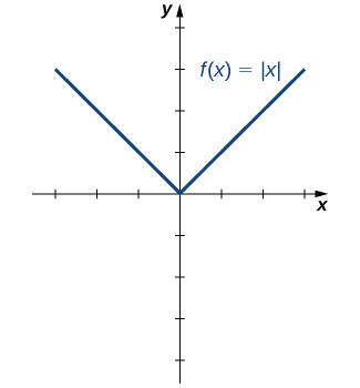
One symmetric function that arises frequently is the absolute value function, written as \(|x|\). The absolute value function is defined as

\[f(x)=\begin{cases} -x, & \text{if }x<0 \\ x, & \text{if } x≥0 \end{cases} \nonumber \]

Some students describe this function by stating that it “makes everything positive.” By the definition of the absolute value function, we see that if \(x<0\), then \(|x|=−x>0,\) and if \(x>0\), then \(|x|=x>0.\) However, for \(x=0,\) \(|x|=0.\) Therefore, it is more accurate to say that for all nonzero inputs, the output is positive, but if \(x=0\), the output \(|x|=0\). We conclude that the range of the absolute value function is \(\{y\,|\,y≥0\}.\) In Figure \(\PageIndex{13}\), we see that the absolute value function is symmetric about the \(y\)-axis and is therefore an even function.

Figure \(\PageIndex{13}\): The graph of \(f(x)=|x|\) is symmetric about the \(y\)-axis.

Example \(\PageIndex{11}\): Working with the Absolute Value Function

Find the domain and range of the function \(f(x)=2|x−3|+4\).

Solution

Since the absolute value function is defined for all real numbers, the domain of this function is \((−∞,∞)\). Since \(|x−3|≥0\) for all \(x\), the function \(f(x)=2|x−3|+4≥4\). Therefore, the range is, at most, the set \(\{y\,|\,y≥4\}.\) To see that the range is, in fact, this whole set, we need to show that for \(y≥4\) there exists a real number \(x\) such that

\(2|x−3|+4=y\)

A real number \(x\) satisfies this equation as long as

\(|x−3|=\frac{1}{2}(y−4)\)

Since \(y≥4\), we know \(y−4≥0\), and thus the right-hand side of the equation is nonnegative, so it is possible that there is a solution. Furthermore,

\(|x−3|=\begin{cases} −(x−3), & \text{if } x<3\\x−3, & \text{if } x≥3\end{cases}\)

Therefore, we see there are two solutions:

\(x=±\frac{1}{2}(y−4)+3\).

The range of this function is \(\{y\,|\,y≥4\}.\)

Exercise \(\PageIndex{11}\): Domain and Range

For the function \(f(x)=|x+2|−4\), find the domain and range.

Hint

\(|x+2|≥0\) for all real numbers \(x\).

Answer

Domain = \((−∞,∞)\), range = \(\{y\,|\,y≥−4\}.\)

Inverse Functions

An inverse function reverses the operation done by a particular function. In other words, whatever a function does, the inverse function undoes it. In this section, we define an inverse function formally and state the necessary conditions for an inverse function to exist. We examine how to find an inverse function and study the relationship between the graph of a function and the graph of its inverse. Then we apply these ideas to define and discuss properties of the inverse trigonometric functions.

Existence of an Inverse Function

We begin with an example. Given a function \(f\) and an output \(y=f(x)\), we are often interested in finding what value or values \(x\) were mapped to \(y\) by \(f\). For example, consider the function \(f(x)=x^3+4\). Since any output \(y=x^3+4\), we can solve this equation for \(x\) to find that the input is \(x=\sqrt[3]{y−4}\). This equation defines \(x\) as a function of \(y\). Denoting this function as \(f^{−1}\), and writing \(x=f^{−1}(y)=\sqrt[3]{y−4}\), we see that for any \(x\) in the domain of \(f,f^{−1}\)\(f(x))=f^{−1}(x^3+4)=x\). Thus, this new function, \(f^{−1}\), “undid” what the original function \(f\) did. A function with this property is called the inverse function of the original function.

Definition: Inverse Functions

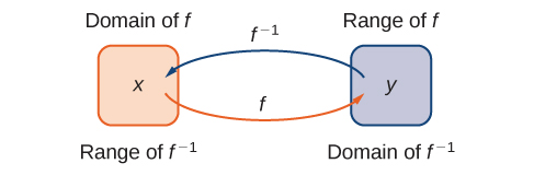
Given a function \(f\) with domain \(D\) and range \(R\), its inverse function (if it exists) is the function \(f^{−1}\) with domain \(R\) and range \(D\) such that \(f^{−1}(y)=x\) if and only if \(f(x)=y\). In other words, for a function \(f\) and its inverse \(f^{−1}\),

\[f^{−1}(f(x))=x \nonumber \]

for all \(x\) in \(D\) and

\[f(f^{−1}(y))=y \nonumber \]

for all \(y\) in \(R\).

Note that \(f^{−1}\) is read as “\(f\) inverse.” Here, the \(−1\) is not used as an exponent so

\[f^{−1}(x)≠ \dfrac{1}{f(x)}. \nonumber \]

Figure \(\PageIndex{1}\)shows the relationship between the domain and range of \(f\) and the domain and range of \(f^{−1}\).

Figure \(\PageIndex{1}\): Given a function \(f\) and its inverse \(f^{−1},f^{−1}(y)=x\) if and only if \(f(x)=y\). The range of \(f\) becomes the domain of \(f^{−1}\) and the domain of \(f\) becomes the range of \(f^{−1}\).

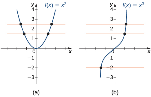
Recall that a function has exactly one output for each input. Therefore, to define an inverse function, we need to map each input to exactly one output. For example, let’s try to find the inverse function for \(f(x)=x^2\). Solving the equation \(y=x^2\) for \(x\), we arrive at the equation \(x=±\sqrt{y}\). This equation does not describe \(x\) as a function of \(y\) because there are two solutions to this equation for every \(y>0\). The problem with trying to find an inverse function for \(f(x)=x^2\) is that two inputs are sent to the same output for each output \(y>0\). The function \(f(x)=x^3+4\) discussed earlier did not have this problem. For that function, each input was sent to a different output. A function that sends each input to a different output is called a one-to-one function.

Definition: One-to-One functions

We say a function \(f\) is a one-to-one function if \(f(x_1)≠f(x_2)\) when \(x_1≠x_2\).

One way to determine whether a function is one-to-one is by looking at its graph. If a function is one-to-one, then no two inputs can be sent to the same output. Therefore, if we draw a horizontal line anywhere in the \(xy\)-plane, according to the horizontal line test, it cannot intersect the graph more than once. We note that the horizontal line test is different from the vertical line test. The vertical line test determines whether a graph is the graph of a function. The horizontal line test determines whether a function is one-to-one (Figure \(\PageIndex{2}\)).

Horizontal Line Test

A function \(f\) is one-to-one if and only if every horizontal line intersects the graph of \(f\) no more than once.

Figure \(\PageIndex{2}\): (a) The function \(f(x)=x^2\) is not one-to-one because it fails the horizontal line test. (b) The function \(f(x)=x^3\) is one-to-one because it passes the horizontal line test.

Example \(\PageIndex{1}\): Determining Whether a Function Is One-to-One

For each of the following functions, use the horizontal line test to determine whether it is one-to-one.

a)

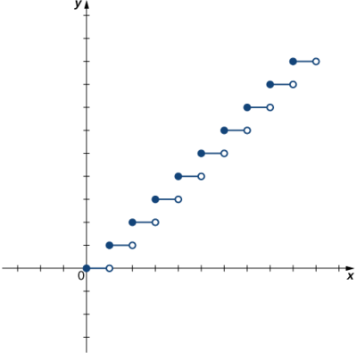
b)

Solution

a) Since the horizontal line \(y=n\) for any integer \(n≥0\) intersects the graph more than once, this function is not one-to-one.

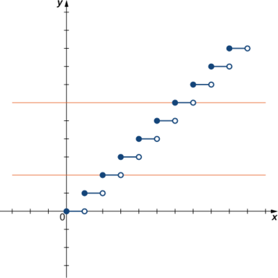
b) Since every horizontal line intersects the graph once (at most), this function is one-to-one.

Exercise \(\PageIndex{1}\)

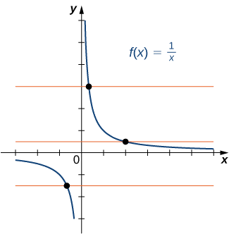
Is the function \(f\) graphed in the following image one-to-one?

Solution

Use the horizontal line test.

Answer

No

Finding a Function’s Inverse

We can now consider one-to-one functions and show how to find their inverses. Recall that a function maps elements in the domain of \(f\) to elements in the range of \(f\). The inverse function maps each element from the range of \(f\) back to its corresponding element from the domain of \(f\). Therefore, to find the inverse function of a one-to-one function \(f\), given any \(y\) in the range of \(f\), we need to determine which \(x\) in the domain of \(f\) satisfies \(f(x)=y\). Since \(f\) is one-to-one, there is exactly one such value \(x\). We can find that value \(x\) by solving the equation \(f(x)=y\) for \(x\). Doing so, we are able to write \(x\) as a function of \(y\) where the domain of this function is the range of \(f\) and the range of this new function is the domain of \(f\). Consequently, this function is the inverse of \(f\), and we write \(x=f^{−1}(y)\). Since we typically use the variable \(x\) to denote the independent variable and y to denote the dependent variable, we often interchange the roles of \(x\) and \(y\), and write \(y=f^{−1}(x)\). Representing the inverse function in this way is also helpful later when we graph a function \(f\) and its inverse \(f^{−1}\) on the same axes.

Problem-Solving Strategy: Finding an Inverse Function

1. Solve the equation \(y=f(x)\) for \(x\).
2. Interchange the variables \(x\) and \(y\) and write \(y=f^{−1}(x)\).

Example \(\PageIndex{2}\): Finding an Inverse Function

Find the inverse for the function \(f(x)=3x−4.\) State the domain and range of the inverse function. Verify that \(f^{−1}(f(x))=x.\)

Solution

Follow the steps outlined in the strategy.

Step 1. If \(y=3x−4,\) then \(3x=y+4\) and \(x=\frac{1}{3}y+\frac{4}{3}.\)

Step 2. Rewrite as \(y=\frac{1}{3}x+\frac{4}{3}\) and let \(y=f^{−1}(x)\).Therefore, \(f^{−1}(x)=\frac{1}{3}x+\frac{4}{3}\).

Since the domain of \(f\) is \((−∞,∞)\), the range of \(f^{−1}\) is \((−∞,∞)\). Since the range of \(f\) is \((−∞,∞)\), the domain of \(f^{−1}\) is \((−∞,∞)\).

You can verify that \(f^{−1}(f(x))=x\) by writing

\(f^{−1}(f(x))=f^{−1}(3x−4)=\frac{1}{3}(3x−4)+\frac{4}{3}=x−\frac{4}{3}+\frac{4}{3}=x.\)

Note that for \(f^{−1}(x)\) to be the inverse of \(f(x)\), both \(f^{−1}(f(x))=x\) and \(f(f^{−1}(x))=x\) for all \(x\) in the domain of the inside function.

Exercise \(\PageIndex{2}\)

Find the inverse of the function \(f(x)=3x/(x−2)\). State the domain and range of the inverse function.

Hint

Use the Problem-Solving Strategy for finding inverse functions.

Answer

\(f^{−1}(x)=\dfrac{2x}{x−3}\). The domain of \(f^{−1}\) is \(\{x\,|\,x≠3\}\). The range of \(f^{−1}\) is \(\{y\,|\,y≠2\}\).

Graphing Inverse Functions

Let’s consider the relationship between the graph of a function \(f\) and the graph of its inverse. Consider the graph of \(f\) shown in Figure \(\PageIndex{3}\) and a point \((a,b)\) on the graph. Since \(b=f(a)\), then \(f^{−1}(b)=a\). Therefore, when we graph \(f^{−1}\), the point \((b,a)\) is on the graph. As a result, the graph of \(f^{−1}\) is a reflection of the graph of \(f\) about the line \(y=x\).

Figure \(\PageIndex{3}\): (a) The graph of this function \(f\) shows point \((a,b)\) on the graph of \(f\). (b) Since \((a,b)\) is on the graph of \(f\), the point \((b,a)\) is on the graph of \(f^{−1}\). The graph of \(f^{−1}\) is a reflection of the graph of \(f\) about the line \(y=x\).

Example \(\PageIndex{3}\): Sketching Graphs of Inverse Functions

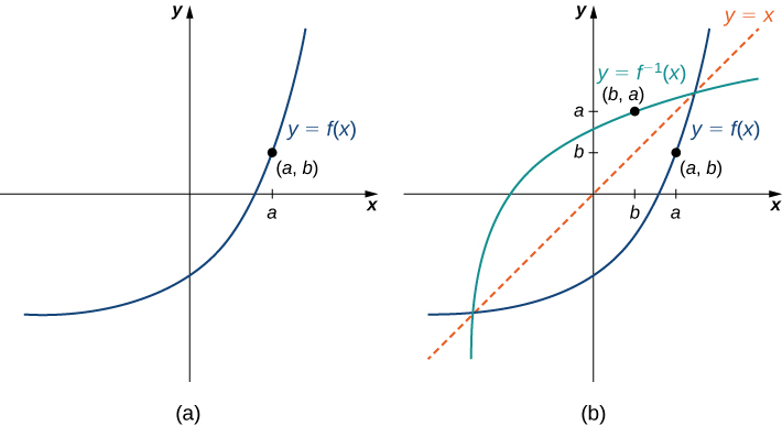
For the graph of \(f\) in the following image, sketch a graph of \(f^{−1}\) by sketching the line \(y=x\) and using symmetry. Identify the domain and range of \(f^{−1}\).

Solution

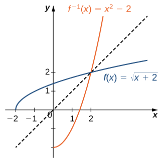
Reflect the graph about the line \(y=x\). The domain of \(f^{−1}\) is \([0,∞)\). The range of \(f^{−1}\) is \([−2,∞)\). By using the preceding strategy for finding inverse functions, we can verify that the inverse function is \(f^{−1}(x)=x^2−2\), as shown in the graph.

Exercise \(\PageIndex{3}\)

Sketch the graph of \(f(x)=2x+3\) and the graph of its inverse using the symmetry property of inverse functions.

Hint

The graphs are symmetric about the line \(y=x\)

Answer

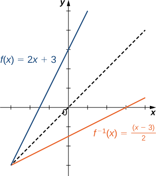
Restricting Domains

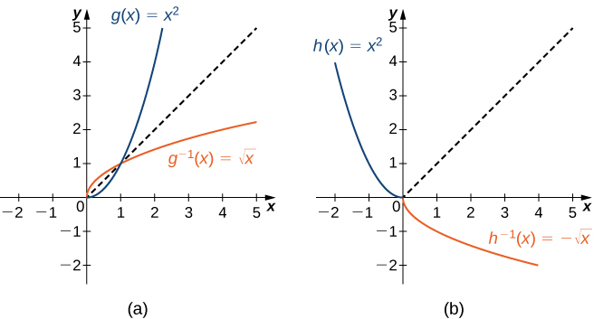
As we have seen, \(f(x)=x^2\) does not have an inverse function because it is not one-to-one. However, we can choose a subset of the domain of \(f\) such that the function is one-to-one. This subset is called a restricted domain. By restricting the domain of \(f\), we can define a new function \(g\) such that the domain of \(g\) is the restricted domain of \(f\) and \(g(x)=f(x)\) for all \(x\) in the domain of \(g\). Then we can define an inverse function for \(g\) on that domain. For example, since \(f(x)=x^2\) is one-to-one on the interval \([0,∞)\), we can define a new function \(g\) such that the domain of \(g\) is \([0,∞)\) and \(g(x)=x^2\) for all \(x\) in its domain. Since \(g\) is a one-to-one function, it has an inverse function, given by the formula \(g^{−1}(x)=\sqrt{x}\). On the other hand, the function \(f(x)=x^2\) is also one-to-one on the domain \((−∞,0]\). Therefore, we could also define a new function \(h\) such that the domain of \(h\) is \((−∞,0]\) and \(h(x)=x^2\) for all \(x\) in the domain of \(h\). Then \(h\) is a one-to-one function and must also have an inverse. Its inverse is given by the formula \(h^{−1}(x)=−\sqrt{x}\) (Figure \(\PageIndex{4}\)).

Figure \(\PageIndex{4}\): (a) For \(g(x)=x^2\) restricted to \([0,∞)\), \(g^{−1}(x)=\sqrt{x}\). (b) For \(h(x)=x^2\) restricted to \((−∞,0]\), \(h^{−1}(x)=−\sqrt{x}\).

Example \(\PageIndex{4}\): Restricting the Domain

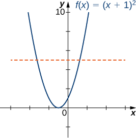
Consider the function \(f(x)=(x+1)^2\).

1. Sketch the graph of \(f\) and use the horizontal line test to show that \(f\) is not one-to-one.
2. Show that \(f\) is one-to-one on the restricted domain \([−1,∞)\). Determine the domain and range for the inverse of \(f\) on this restricted domain and find a formula for \(f^{−1}\).

Solution

a) The graph of \(f\) is the graph of \(y=x^2\) shifted left \(1\) unit. Since there exists a horizontal line intersecting the graph more than once, \(f\) is not one-to-one.

b) On the interval \([−1,∞),\;f\) is one-to-one.

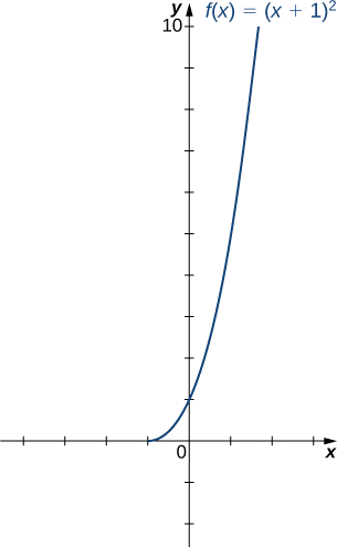
The domain and range of \(f^{−1}\) are given by the range and domain of \(f\), respectively. Therefore, the domain of \(f^{−1}\) is \([0,∞)\) and the range of \(f^{−1}\) is \([−1,∞)\). To find a formula for \(f^{−1}\), solve the equation \(y=(x+1)^2\) for \(x.\) If \(y=(x+1)^2\), then \(x=−1±\sqrt{y}\). Since we are restricting the domain to the interval where \(x≥−1\), we need \(±\sqrt{y}≥0\). Therefore, \(x=−1+\sqrt{y}\). Interchanging \(x\) and \(y\), we write \(y=−1+\sqrt{x}\) and conclude that \(f^{−1}(x)=−1+\sqrt{x}\).

Exercise \(\PageIndex{4}\)

Consider \(f(x)=1/x^2\) restricted to the domain \((−∞,0)\). Verify that \(f\) is one-to-one on this domain. Determine the domain and range of the inverse of \(f\) and find a formula for \(f^{−1}\).

Hint

The domain and range of \(f^{−1}\) is given by the range and domain of \(f\), respectively. To find \(f^{−1}\), solve \(y=1/x^2\) for \(x\).

Answer

The domain of \(f^{−1}\) is \((0,∞)\). The range of \(f^{−1}\) is \((−∞,0)\). The inverse function is given by the formula \(f^{−1}(x)=−1/\sqrt{x}\).

Key Concepts

• For a function to have an inverse, the function must be one-to-one. Given the graph of a function, we can determine whether the function is one-to-one by using the horizontal line test.
• If a function is not one-to-one, we can restrict the domain to a smaller domain where the function is one-to-one and then define the inverse of the function on the smaller domain.
• For a function \(f\) and its inverse \(f^{−1},\, f(f^{−1}(x))=x\) for all \(x\) in the domain of \(f^{−1}\) and \(f^{−1}(f(x))=x\) for all \(x\) in the domain of \(f\).
• Since the trigonometric functions are periodic, we need to restrict their domains to define the inverse trigonometric functions.
• The graph of a function \(f\) and its inverse \(f^{−1}\) are symmetric about the line \(y=x.\)

Key Equations

• Inverse function

\(f^{−1}(f(x))=x\) for all \(x\) in \(D,\) and \(f(f^{−1}(y))=y\) for all \(y\) in \(R\).

Glossary

horizontal line test

a function \(f\) is one-to-one if and only if every horizontal line intersects the graph of \(f\), at most, once

inverse function

for a function \(f\), the inverse function \(f^{−1}\) satisfies \(f^{−1}(y)=x\) if \(f(x)=y\)

inverse trigonometric functions

the inverses of the trigonometric functions are defined on restricted domains where they are one-to-one functions

one-to-one function

a function \(f\) is one-to-one if \(f(x_1)≠f(x_2)\) if \(x_1≠x_2\)

restricted domain

a subset of the domain of a function \(f\)

Key Concepts

• A function is a mapping from a set of inputs to a set of outputs with exactly one output for each input.
• If no domain is stated for a function \(y=f(x),\) the domain is considered to be the set of all real numbers \(x\) for which the function is defined.
• When sketching the graph of a function \(f,\) each vertical line may intersect the graph, at most, once.
• A function may have any number of zeros, but it has, at most, one \(y\)-intercept.
• To define the composition \(g∘f\), the range of \(f\) must be contained in the domain of \(g\).
• Even functions are symmetric about the \(y\)-axis whereas odd functions are symmetric about the origin.

Key Equations

• Composition of two functions

\((g∘f)(x)=g\big(f(x)\big)\)

• Absolute value function

\(f(x)=\begin{cases}−x, & \text{if } x<0\\x, & \text{if } x≥0\end{cases}\)

Glossary

absolute value function

\(f(x)=\begin{cases}−x, & \text{if } x<0\\x, & \text{if } x≥0\end{cases}\)

composite function

given two functions \(f\) and \(g\), a new function, denoted \(g∘f\), such that \((g∘f)(x)=g(f(x))\)

decreasing on the interval \(I\)

a function decreasing on the interval \(I\) if, for all \(x_1,\,x_2∈I,\;f(x_1)≥f(x_2)\) if \(x_1<x_2\)

dependent variable

the output variable for a function

domain

the set of inputs for a function

even function

a function is even if \(f(−x)=f(x)\) for all \(x\) in the domain of \(f\)

function

a set of inputs, a set of outputs, and a rule for mapping each input to exactly one output

graph of a function

the set of points \((x,y)\) such that \(x\) is in the domain of \(f\) and \(y=f(x)\)

increasing on the interval \(I\)

a function increasing on the interval \(I\) if for all \(x_1,\,x_2∈I,\;f(x_1)≤f(x_2)\) if \(x_1<x_2\)

independent variable

the input variable for a function

odd function

a function is odd if \(f(−x)=−f(x)\) for all \(x\) in the domain of \(f\)

range

the set of outputs for a function

symmetry about the origin

the graph of a function \(f\) is symmetric about the origin if \((−x,−y)\) is on the graph of \(f\) whenever \((x,y)\) is on the graph

symmetry about the \(y\)-axis

the graph of a function \(f\) is symmetric about the \(y\)-axis if \((−x,y)\) is on the graph of \(f\) whenever \((x,y)\) is on the graph

table of values

a table containing a list of inputs and their corresponding outputs

vertical line test

given the graph of a function, every vertical line intersects the graph, at most, once

zeros of a function

when a real number \(x\) is a zero of a function \(f,\;f(x)=0\)