2.7.19: Applications- Rates of Change, Linear Approximation, Calculating Uncertainty, Maxima and Minima, Optimization

Learning Objectives

• Determine a new value of a quantity from the old value and the amount of change.
• Calculate the average rate of change and explain how it differs from the instantaneous rate of change.
• Apply rates of change to displacement, velocity, and acceleration of an object moving along a straight line.
• Predict the future population from the present value and the population growth rate.
• Use derivatives to calculate marginal cost and revenue in a business situation.
• Describe the linear approximation to a function at a point.
• Write the linearization of a given function.
• Draw a graph that illustrates the use of differentials to approximate the change in a quantity.
• Calculate the relative uncertainty and percentage uncertainty in using a differential approximation.
• Define absolute extrema.
• Define local extrema.
• Explain how to find the critical points of a function over a closed interval.
• Describe how to use critical points to locate absolute extrema over a closed interval.
• Set up and solve optimization problems in several applied fields.

In this section we look at some applications of the derivative in Physics.

Motion along a Line

Another use for the derivative is to analyze motion along a line. We have described velocity as the rate of change of position. If we take the derivative of the velocity, we can find the acceleration, or the rate of change of velocity. It is also important to introduce the idea of speed, which is the magnitude of velocity. Thus, we can state the following mathematical definitions.

Definition

Let \(s(t)\) be a function giving the position of an object at time t.

• The velocity of the object at time \(t\) is given by \(v(t)=s′(t)\).
• The speed of the object at time \(t\) is given by \(|v(t)|\).
• The acceleration of the object at \(t\) is given by \(a(t)=v′(t)=s''(t)\).

Example \(\PageIndex{2}\): Comparing Instantaneous Velocity and Average Velocity

A ball is dropped from a height of 64 feet. Its height above ground (in feet) \(t\) seconds later is given by \(s(t)=−16t^2+64\).

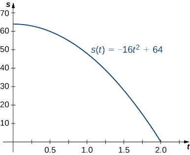
1. What is the instantaneous velocity of the ball when it hits the ground?
2. What is the average velocity during its fall?

Solution

The first thing to do is determine how long it takes the ball to reach the ground. To do this, set \(s(t)=0\). Solving \(−16t^2+64=0\), we get \(t=2\), so it takes 2 seconds for the ball to reach the ground.

1. The instantaneous velocity of the ball as it strikes the ground is \(v(2)\). Since \(v(t)=s′(t)=−32t\), we obtain \(v(t)=−64\) ft/s.
2. The average velocity of the ball during its fall is

\(v_{ave}=\frac{s(2)−s(0)}{2−0}=\frac{0−64}{2}=−32\) ft/s.

Example \(\PageIndex{3}\): Interpreting the Relationship between \(v(t)\) and \(a(t)\)

A particle moves along a coordinate axis in the positive direction to the right. Its position at time \(t\) is given by \(s(t)=t^3−4t+2\). Find \(v(1)\) and \(a(1)\) and use these values to answer the following questions.

1. Is the particle moving from left to right or from right to left at time \(t=1\)?
2. Is the particle speeding up or slowing down at time \(t=1\)?

Solution

Begin by finding \(v(t)\) and \(a(t)\).

\(v(t) = s'(t) = 3t^2 - 4\) and \(a(t)=v′(t)=s''(t)=6t\).

Evaluating these functions at \(t=1\), we obtain \(v(1)=−1\) and \(a(1)=6\).

1. Because \(v(1)<0\), the particle is moving from right to left.
2. Because \(v(1)<0\) and \(a(1)>0\), velocity and acceleration are acting in opposite directions. In other words, the particle is being accelerated in the direction opposite the direction in which it is traveling, causing \(|v(t)|\) to decrease. The particle is slowing down.

Example \(\PageIndex{4}\): Position and Velocity

The position of a particle moving along a coordinate axis is given by \(s(t)=t^3−9t^2+24t+4,\; t≥0.\)

1. Find \(v(t)\).
2. At what time(s) is the particle at rest?
3. On what time intervals is the particle moving from left to right? From right to left?
4. Use the information obtained to sketch the path of the particle along a coordinate axis.

Solution

a. The velocity is the derivative of the position function:

\(v(t)=s′(t)=3t^2−18t+24.\)

b. The particle is at rest when \(v(t)=0\), so set \(3t^2−18t+24=0\). Factoring the left-hand side of the equation produces \(3(t−2)(t−4)=0\). Solving, we find that the particle is at rest at \(t=2\) and \(t=4\).

c. The particle is moving from left to right when \(v(t)>0\) and from right to left when \(v(t)<0\). Figure \(\PageIndex{2}\) gives the analysis of the sign of \(v(t)\) for \(t≥0\), but it does not represent the axis along which the particle is moving.

Figure \(\PageIndex{2}\):The sign of \(v(t)\) determines the direction of the particle.

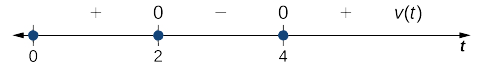
• Since \(3t^2−18t+24>0\) on \([0,2)∪(4,+∞)\), the particle is moving from left to right on these intervals.
• Since \(3t^2−18t+24<0\) on \((2,4)\), the particle is moving from right to left on this interval.

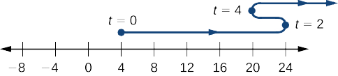
d. Before we can sketch the graph of the particle, we need to know its position at the time it starts moving \((t=0)\) and at the times that it changes direction \((t=2,4)\). We have \(s(0)=4\), \(s(2)=24\), and \(s(4)=20\). This means that the particle begins on the coordinate axis at \(4\) and changes direction at \(24\) and \(20\) on the coordinate axis. The path of the particle is shown on a coordinate axis in Figure \(\PageIndex{3}\).

Figure \(\PageIndex{3}\): The path of the particle can be determined by analyzing \(v(t)\).

Exercise \(\PageIndex{2}\)

A particle moves along a coordinate axis. Its position at time \(t\) is given by \(s(t)=t^2−5t+1\). Is the particle moving from right to left or from left to right at time \(t=3\)?

Hint

Find \(v(3)\) and look at the sign.

Answer

left to right

Linear Approximation of a Function at a Point

Consider a function \(f\) that is differentiable at a point \(x=a\). Recall that the tangent line to the graph of \(f\) at \(a\) is given by the equation

\[y=f(a)+f'(a)(x−a). \nonumber \]

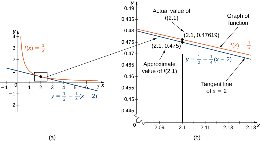
For example, consider the function \(f(x)=\frac{1}{x}\) at \(a=2\). Since \(f\) is differentiable at \(x=2\) and \(f'(x)=−\frac{1}{x^2}\), we see that \(f'(2)=−\frac{1}{4}\). Therefore, the tangent line to the graph of \(f\) at \(a=2\) is given by the equation

\[y=\frac{1}{2}−\frac{1}{4}(x−2). \nonumber \]

Figure \(\PageIndex{1a}\) shows a graph of \(f(x)=\frac{1}{x}\) along with the tangent line to \(f\) at \(x=2\). Note that for \(x\) near \(2\), the graph of the tangent line is close to the graph of \(f\). As a result, we can use the equation of the tangent line to approximate \(f(x)\) for \(x\) near \(2\). For example, if \(x=2.1\), the \(y\) value of the corresponding point on the tangent line is

\[y=\frac{1}{2}−\frac{1}{4}(2.1−2)=0.475. \nonumber \]

The actual value of \(f(2.1)\) is given by

\[f(2.1)=\frac{1}{2.1}≈0.47619. \nonumber \]

Therefore, the tangent line gives us a fairly good approximation of \(f(2.1)\) (Figure \(\PageIndex{1b}\)). However, note that for values of \(x\) far from \(2\), the equation of the tangent line does not give us a good approximation. For example, if \(x=10\), the \(y\)-value of the corresponding point on the tangent line is

\[y=\frac{1}{2}−\frac{1}{4}(10−2)=\frac{1}{2}−2=−1.5, \nonumber \]

whereas the value of the function at \(x=10\) is \(f(10)=0.1.\)

Figure \(\PageIndex{1}\): (a) The tangent line to \(f(x)=1/x\) at \(x=2\) provides a good approximation to \(f\) for \(x\) near \(2\). (b) At \(x=2.1\), the value of \(y\) on the tangent line to \(f(x)=1/x\) is \(0.475\). The actual value of \(f(2.1)\) is \(1/2.1\), which is approximately \(0.47619\).

In general, for a differentiable function \(f\), the equation of the tangent line to \(f\) at \(x=a\) can be used to approximate \(f(x)\) for \(x\) near \(a\). Therefore, we can write

\(f(x)≈f(a)+f'(a)(x−a)\) for \(x\) near \(a\).

We call the linear function

\[L(x)=f(a)+f'(a)(x−a) \label{linearapprox} \]

the linear approximation, or tangent line approximation, of \(f\) at \(x=a\). This function \(L\) is also known as the linearization of \(f\) at \(x=a.\)

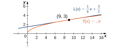
To show how useful the linear approximation can be, we look at how to find the linear approximation for \(f(x)=\sqrt{x}\) at \(x=9.\)

Example \(\PageIndex{1}\): Linear Approximation of \(\sqrt{x}\)

Find the linear approximation of \(f(x)=\sqrt{x}\) at \(x=9\) and use the approximation to estimate \(\sqrt{9.1}\).

Solution

Since we are looking for the linear approximation at \(x=9,\) using Equation \ref{linearapprox} we know the linear approximation is given by

\[L(x)=f(9)+f'(9)(x−9). \nonumber \]

We need to find \(f(9)\) and \(f'(9).\)

\(f(x)=\sqrt{x}⇒f(9)=\sqrt{9}=3\)

\(f'(x)=\frac{1}{2\sqrt{x}}⇒f'(9)=\frac{1}{2\sqrt{9}}=\frac{1}{6}\)

Therefore, the linear approximation is given by Figure \(\PageIndex{2}\).

\[L(x)=3+\frac{1}{6}(x−9) \nonumber \]

Using the linear approximation, we can estimate \(\sqrt{9.1}\) by writing

\[\sqrt{9.1}=f(9.1)≈L(9.1)=3+\frac{1}{6}(9.1−9)≈3.0167. \nonumber \]

Figure \(\PageIndex{2}\): The local linear approximation to \(f(x)=\sqrt{x}\) at \(x=9\) provides an approximation to \(f\) for \(x\) near \(9\).

Analysis

Using a calculator, the value of \(\sqrt{9.1}\) to four decimal places is \(3.0166\). The value given by the linear approximation, \(3.0167\), is very close to the value obtained with a calculator, so it appears that using this linear approximation is a good way to estimate \(\sqrt{x}\), at least for x near \(9\). At the same time, it may seem odd to use a linear approximation when we can just push a few buttons on a calculator to evaluate \(\sqrt{9.1}\). However, how does the calculator evaluate \(\sqrt{9.1}\)? The calculator uses an approximation! In fact, calculators and computers use approximations all the time to evaluate mathematical expressions; they just use higher-degree approximations.

Exercise \(\PageIndex{1}\)

Find the local linear approximation to \(f(x)=\sqrt[3]{x}\) at \(x=8\). Use it to approximate \(\sqrt[3]{8.1}\) to five decimal places.

Hint

\(L(x)=f(a)+f'(a)(x−a)\)

Answer

\(L(x)=2+\frac{1}{12}(x−8);\) \(2.00833\)

Example \(\PageIndex{2}\): Linear Approximation of \(\sin x \)

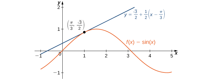
Find the linear approximation of \(f(x)=\sin x \) at \(x=\frac{π}{3}\) and use it to approximate \(\sin(62°).\)

Solution

First we note that since \(\frac{π}{3}\) rad is equivalent to \(60°\), using the linear approximation at \(x=π/3\) seems reasonable. The linear approximation is given by

\(L(x)=f(\frac{π}{3})+f'(\frac{π}{3})(x−\frac{π}{3}).\)

We see that

\(f(x)=\sin x ⇒f(\frac{π}{3})=\sin(\frac{π}{3})=\frac{\sqrt{3}}{2}\)

\(f'(x)=\cos x ⇒f'(\frac{π}{3})=\cos(\frac{π}{3})=\frac{1}{2}\)

Therefore, the linear approximation of \(f\) at \(x=π/3\) is given by Figure \(\PageIndex{3}\).

\(L(x)=\frac{\sqrt{3}}{2}+\frac{1}{2}(x−\frac{π}{3})\)

To estimate \(\sin(62°)\) using \(L\), we must first convert \(62°\) to radians. We have \(62°=\frac{62π}{180}\) radians, so the estimate for \(\sin(62°)\) is given by

\(\sin(62°)=f(\frac{62π}{180})≈L(\frac{62π}{180})=\frac{\sqrt{3}}{2}+\frac{1}{2}(\frac{62π}{180}−\frac{π}{3})=\frac{\sqrt{3}}{2}+\frac{1}{2}(\frac{2π}{180})=\frac{\sqrt{3}}{2}+\frac{π}{180}≈0.88348.\)

Figure \(\PageIndex{3}\): The linear approximation to \(f(x)=\sin x \) at \(x=π/3\) provides an approximation to \(\sin x \) for \(x\) near \(π/3.\)

Exercise \(\PageIndex{2}\)

Find the linear approximation for \(f(x)=\cos x \) at \(x=\frac{π}{2}.\)

Hint

\(L(x)=f(a)+f'(a)(x−a)\)

Answer

\(L(x)=−x+\frac{π}{2}\)

Linear approximations may be used in estimating roots and powers. In the next example, we find the linear approximation for \(f(x)=(1+x)^n\) at \(x=0\), which can be used to estimate roots and powers for real numbers near \(1\). The same idea can be extended to a function of the form \(f(x)=(m+x)^n\) to estimate roots and powers near a different number \(m\).

Example \(\PageIndex{3}\): Approximating Roots and Powers

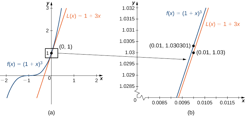
Find the linear approximation of \(f(x)=(1+x)^n\) at \(x=0\). Use this approximation to estimate \((1.01)^3.\)

Solution

The linear approximation at \(x=0\) is given by

\(L(x)=f(0)+f'(0)(x−0).\)

Because

\(f(x)=(1+x)^n⇒f(0)=1\)

\(f'(x)=n(1+x)^{n−1}⇒f'(0)=n,\)

the linear approximation is given by Figure \(\PageIndex{4a}\).

\(L(x)=1+n(x−0)=1+nx\)

We can approximate \((1.01)^3\) by evaluating \(L(0.01)\) when \(n=3\). We conclude that

\((1.01)^3=f(1.01)≈L(1.01)=1+3(0.01)=1.03.\)

Figure \(\PageIndex{4}\): (a) The linear approximation of \(f(x)\) at \(x=0\) is \(L(x)\). (b) The actual value of \(1.01^3\) is \(1.030301\). The linear approximation of \(f(x)\) at \(x=0\) estimates \(1.01^3\) to be \(1.03\).

Exercise \(\PageIndex{3}\)

Find the linear approximation of \(f(x)=(1+x)^4\) at \(x=0\) without using the result from the preceding example.

Hint

\(f'(x)=4(1+x)^3\)

Answer

\(L(x)=1+4x\)

Differentials

We have seen that linear approximations can be used to estimate function values. They can also be used to estimate the amount a function value changes as a result of a small change in the input. To discuss this more formally, we define a related concept: differentials. Differentials provide us with a way of estimating the amount a function changes as a result of a small change in input values.

When we first looked at derivatives, we used the Leibniz notation \(dy/dx\) to represent the derivative of \(y\) with respect to \(x\). Although we used the expressions \(dy\) and \(dx\) in this notation, they did not have meaning on their own. Here we see a meaning to the expressions \(dy\) and \(dx\). Suppose \(y=f(x)\) is a differentiable function. Let \(dx\) be an independent variable that can be assigned any nonzero real number, and define the dependent variable \(dy\) by

\[dy=f'(x)\,dx. \label{diffeq} \]

It is important to notice that \(dy\) is a function of both \(x\) and \(dx\). The expressions \(dy\) and \(dx\) are called differentials. We can divide both sides of Equation \ref{diffeq} by \(dx,\) which yields

\[\frac{dy}{dx}=f'(x). \label{inteq} \]

This is the familiar expression we have used to denote a derivative. Equation \ref{inteq} is known as the differential form of Equation \ref{diffeq}.

Example \(\PageIndex{4}\): Computing Differentials

For each of the following functions, find \(dy\) and evaluate when \(x=3\) and \(dx=0.1.\)

1. \(y=x^2+2x\)
2. \(y=\cos x \)

Solution

The key step is calculating the derivative. When we have that, we can obtain \(dy\) directly.

a. Since \(f(x)=x^2+2x,\) we know \(f'(x)=2x+2\), and therefore

\(dy=(2x+2)\,dx.\)

When \(x=3\) and \(dx=0.1,\)

\(dy=(2⋅3+2)(0.1)=0.8.\)

b. Since \(f(x)=\cos x , f'(x)=−\sin(x).\) This gives us

\(dy=−\sin x \,dx.\)

When \(x=3\) and \(dx=0.1,\)

\(dy=−\sin(3)(0.1)=−0.1\sin(3).\)

Exercise \(\PageIndex{4}\)

For \(y=e^{x^2}\), find \(dy\).

Hint

\(dy=f'(x)\,dx\)

Answer

\(dy=2xe^{x^2}dx\)

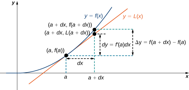
We now connect differentials to linear approximations. Differentials can be used to estimate the change in the value of a function resulting from a small change in input values. Consider a function \(f\) that is differentiable at point \(a\). Suppose the input \(x\) changes by a small amount. We are interested in how much the output \(y\) changes. If \(x\) changes from \(a\) to \(a+dx\), then the change in \(x\) is \(dx\) (also denoted \(Δx\)), and the change in \(y\) is given by

\[Δy=f(a+dx)−f(a). \nonumber \]

Instead of calculating the exact change in \(y\), however, it is often easier to approximate the change in \(y\) by using a linear approximation. For \(x\) near \(a, f(x)\) can be approximated by the linear approximation (Equation \ref{linearapprox})

\[L(x)=f(a)+f'(a)(x−a). \nonumber \]

Therefore, if \(dx\) is small,

\[f(a+dx)≈L(a+dx)=f(a)+f'(a)(a+dx−a). \nonumber \]

That is,

\[f(a+dx)−f(a)≈L(a+dx)−f(a)=f'(a)\,dx. \nonumber \]

In other words, the actual change in the function \(f\) if \(x\) increases from \(a\) to \(a+dx\) is approximately the difference between \(L(a+dx)\) and \(f(a)\), where \(L(x)\) is the linear approximation of \(f\) at \(a\). By definition of \(L(x)\), this difference is equal to \(f'(a)\,dx\). In summary,

\[Δy=f(a+dx)−f(a)≈L(a+dx)−f(a)=f'(a)\,dx=dy. \nonumber \]

Therefore, we can use the differential \(dy=f'(a)\,dx\) to approximate the change in \(y\) if \(x\) increases from \(x=a\) to \(x=a+dx\). We can see this in the following graph.

Figure \(\PageIndex{5}\): The differential \(dy=f'(a)\,dx\) is used to approximate the actual change in \(y\) if \(x\) increases from \(a\) to \(a+dx\).

We now take a look at how to use differentials to approximate the change in the value of the function that results from a small change in the value of the input. Note the calculation with differentials is much simpler than calculating actual values of functions and the result is very close to what we would obtain with the more exact calculation.

Example \(\PageIndex{5}\): Approximating Change with Differentials

Let \(y=x^2+2x.\) Compute \(Δy\) and \(dy\) at \(x=3\) if \(dx=0.1.\)

Solution

The actual change in \(y\) if \(x\) changes from \(x=3\) to \(x=3.1\) is given by

\(Δy=f(3.1)−f(3)=[(3.1)^2+2(3.1)]−[3^2+2(3)]=0.81.\)

The approximate change in \(y\) is given by \(dy=f'(3)\,dx\). Since \(f'(x)=2x+2,\) we have

\(dy=f'(3)\,dx=(2(3)+2)(0.1)=0.8.\)

Exercise \(\PageIndex{5}\)

For \(y=x^2+2x,\) find \(Δy\) and \(dy\) at \(x=3\) if \(dx=0.2.\)

Hint

\(dy=f'(3)\,dx, \;Δy=f(3.2)−f(3)\)

Answer

\(dy=1.6, \; Δy=1.64\)

Calculating the Amount of Uncertainty

Any type of measurement is prone to a certain amount of uncertainty. In many applications, certain quantities are calculated based on measurements. For example, the area of a circle is calculated by measuring the radius of the circle. An uncertainty in the measurement of the radius leads to an uncertainty in the computed value of the area. Here we examine this type of uncertainty and study how differentials can be used to estimate the uncertainty.

Consider a function \(f\) with an input that is a measured quantity. Suppose the exact value of the measured quantity is \(a\), but the measured value is \(a+dx\). We say the measurement uncertainty is \(dx\) (or \(Δx\)). As a result, an uncertainty occurs in the calculated quantity \(f(x)\). This type of uncertainty is known as a propagated uncertainty and is given by

\[Δy=f(a+dx)−f(a). \nonumber \]

Since all measurements are prone to some degree of uncertainty, we do not know the exact value of a measured quantity, so we cannot calculate the propagated uncertainty exactly. However, given an estimate of the accuracy of a measurement, we can use differentials to approximate the propagated uncertainty \(Δy.\) Specifically, if \(f\) is a differentiable function at \(a\),the propagated uncertainty is

\[Δy≈dy=f'(a)\,dx. \nonumber \]

Unfortunately, we do not know the exact value \(a.\) However, we can use the measured value \(a+dx,\) and estimate

\[Δy≈dy≈f'(a+dx)\,dx. \nonumber \]

In the next example, we look at how differentials can be used to estimate the uncertainty in calculating the volume of a box if we assume the measurement of the side length is made with a certain amount of accuracy.

Example \(\PageIndex{6}\): Volume of a Cube

Suppose the side length of a cube is measured to be \(5\) cm with an accuracy of \(0.1\) cm.

1. Use differentials to estimate the uncertainty in the computed volume of the cube.
2. Compute the volume of the cube if the side length is (i) \(4.9\) cm and (ii) \(5.1\) cm to compare the estimated uncertainty with the actual potential uncertainty.

Solution

a. The measurement of the side length is accurate to within \(±0.1\) cm. Therefore,

\(−0.1≤dx≤0.1.\)

The volume of a cube is given by \(V=x^3\), which leads to

\(dV=3x^2dx.\)

Using the measured side length of \(5\) cm, we can estimate that

\(−3(5)^2(0.1)≤dV≤3(5)^2(0.1).\)

Therefore,

\(−7.5≤dV≤7.5.\)

b. If the side length is actually \(4.9\) cm, then the volume of the cube is

\(V(4.9)=(4.9)^3=117.649\text{cm}^3.\)

If the side length is actually \(5.1\) cm, then the volume of the cube is

\(V(5.1)=(5.1)^3=132.651\text{cm}^3.\)

Therefore, the actual volume of the cube is between \(117.649\) and \(132.651\). Since the side length is measured to be 5 cm, the computed volume is \(V(5)=5^3=125.\) Therefore, the uncertainty in the computed volume is

\(117.649−125≤ΔV≤132.651−125.\)

That is,

\(−7.351≤ΔV≤7.651.\)

We see the estimated uncertainty \(dV\) is relatively close to the actual potential uncertainty in the computed volume.

Exercise \(\PageIndex{6}\)

Estimate the uncertainty in the computed volume of a cube if the side length is measured to be \(6\) cm with an accuracy of \(0.2\) cm.

Hint

\(dV=3x^2dx\)

Answer

The volume measurement is accurate to within \(21.6\,\text{cm}^3\).

The measurement uncertainty \(dx\ (=Δx)\) and the propagated uncertainty \(Δy\) are absolute uncertaintys. We are typically interested in the size of an uncertainty relative to the size of the quantity being measured or calculated. Given an absolute uncertainty \(Δq\) for a particular quantity, we define the relative uncertainty as \(\frac{Δq}{q}\), where \(q\) is the actual value of the quantity. The percentage uncertainty is the relative uncertainty expressed as a percentage. For example, if we measure the height of a ladder to be \(63\) in. when the actual height is \(62\) in., the absolute uncertainty is 1 in. but the relative uncertainty is \(\frac{1}{62}=0.016\), or \(1.6\%\). By comparison, if we measure the width of a piece of cardboard to be \(8.25\) in. when the actual width is \(8\) in., our absolute uncertainty is \(\frac{1}{4}\) in., whereas the relative uncertainty is \(\frac{0.25}{8}=\frac{1}{32}\), or \(3.1\%.\) Therefore, the percentage uncertainty in the measurement of the cardboard is larger, even though \(0.25\) in. is less than \(1\) in.

Example \(\PageIndex{7}\): Relative and Percentage uncertainty

An astronaut using a camera measures the radius of Earth as \(4000\) mi with an uncertainty of \(±80\) mi. Let’s use differentials to estimate the relative and percentage uncertainty of using this radius measurement to calculate the volume of Earth, assuming the planet is a perfect sphere.

Solution: If the measurement of the radius is accurate to within \(±80,\) we have

\(−80≤dr≤80.\)

Since the volume of a sphere is given by \(V=(\frac{4}{3})πr^3,\) we have

\(dV=4πr^2dr.\)

Using the measured radius of \(4000\) mi, we can estimate

\(−4π(4000)^2(80)≤dV≤4π(4000)^2(80).\)

To estimate the relative uncertainty, consider \(\dfrac{dV}{V}\). Since we do not know the exact value of the volume \(V\), use the measured radius \(r=4000\) mi to estimate \(V\). We obtain \(V≈(\frac{4}{3})π(4000)^3\). Therefore the relative uncertainty satisfies

\(\frac{−4π(4000)^2(80)}{4π(4000)^3/3}≤\dfrac{dV}{V}≤\frac{4π(4000)^2(80)}{4π(4000)^3/3},\)

which simplifies to

\(−0.06≤\dfrac{dV}{V}≤0.06.\)

The relative uncertainty is \(0.06\) and the percentage uncertainty is \(6\%\).

Exercise \(\PageIndex{7}\)

Determine the percentage uncertainty if the radius of Earth is measured to be \(3950\) mi with an uncertainty of \(±100\) mi.

Hint

Use the fact that \(dV=4πr^2dr\) to find \(dV/V\).

Answer

\(7.6\%\)

Absolute Extrema

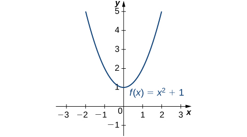
Consider the function \(f(x)=x^2+1\) over the interval \((−∞,∞)\). As \(x→±∞, f(x)→∞\). Therefore, the function does not have a largest value. However, since \(x^2+1≥1\) for all real numbers \(x\) and \(x^2+1=1\) when \(x=0\), the function has a smallest value, \(1\), when \(x=0\). We say that \(1\) is the absolute minimum of \(f(x)=x^2+1\) and it occurs at \(x=0\). We say that \(f(x)=x^2+1\) does not have an absolute maximum (Figure \(\PageIndex{1}\)).

Figure \(\PageIndex{1}\): The given function has an absolute minimum of \(1\) at \(x=0\). The function does not have an absolute maximum.

Definition: Absolute Extrema

Let \(f\) be a function defined over an interval \(I\) and let \(c∈I\). We say \(f\) has an absolute maximum on \(I\) at \(c\) if \(f(c)≥f(x)\) for all \(x∈I\). We say \(f\) has an absolute minimum on \(I\) at \(c\) if \(f(c)≤f(x)\) for all \(x∈I\). If \(f\) has an absolute maximum on \(I\) at \(c\) or an absolute minimum on \(I\) at \(c\), we say \(f\) has an absolute extremum on \(I\) at \(c\).

Before proceeding, let’s note two important issues regarding this definition. First, the term absolute here does not refer to absolute value. An absolute extremum may be positive, negative, or zero. Second, if a function \(f\) has an absolute extremum over an interval \(I\) at \(c\), the absolute extremum is \(f(c)\). The real number \(c\) is a point in the domain at which the absolute extremum occurs. For example, consider the function \(f(x)=1/(x^2+1)\) over the interval \((−∞,∞)\). Since

\[f(0)=1≥\frac{1}{x^2+1}=f(x) \nonumber \]

for all real numbers \(x\), we say \(f\) has an absolute maximum over \((−∞,∞)\) at \(x=0\). The absolute maximum is \(f(0)=1\). It occurs at \(x=0\), as shown in Figure \(\PageIndex{2}\)(b).

A function may have both an absolute maximum and an absolute minimum, just one extremum, or neither. Figure \(\PageIndex{2}\) shows several functions and some of the different possibilities regarding absolute extrema. However, the following theorem, called the Extreme Value Theorem, guarantees that a continuous function \(f\) over a closed, bounded interval \([a,b]\) has both an absolute maximum and an absolute minimum.

Figure \(\PageIndex{2}\): Graphs (a), (b), and (c) show several possibilities for absolute extrema for functions with a domain of \((−∞,∞).\) Graphs (d), (e), and (f) show several possibilities for absolute extrema for functions with a domain that is a bounded interval.

Theorem \(\PageIndex{1}\): Extreme Value Theorem

If \(f\) is a continuous function over the closed, bounded interval \([a,b]\), then there is a point in \([a,b]\) at which \(f\) has an absolute maximum over \([a,b]\) and there is a point in \([a,b]\) at which \(f\) has an absolute minimum over \([a,b]\).

The proof of the extreme value theorem is beyond the scope of this text. Typically, it is proved in a course on real analysis. There are a couple of key points to note about the statement of this theorem. For the extreme value theorem to apply, the function must be continuous over a closed, bounded interval. If the interval \(I\) is open or the function has even one point of discontinuity, the function may not have an absolute maximum or absolute minimum over \(I\). For example, consider the functions shown in Figure \(\PageIndex{2}\) (d), (e), and (f). All three of these functions are defined over bounded intervals. However, the function in graph (e) is the only one that has both an absolute maximum and an absolute minimum over its domain. The extreme value theorem cannot be applied to the functions in graphs (d) and (f) because neither of these functions is continuous over a closed, bounded interval. Although the function in graph (d) is defined over the closed interval \([0,4]\), the function is discontinuous at \(x=2\). The function has an absolute maximum over \([0,4]\) but does not have an absolute minimum. The function in graph (f) is continuous over the half-open interval \([0,2)\), but is not defined at \(x=2\), and therefore is not continuous over a closed, bounded interval. The function has an absolute minimum over \([0,2)\), but does not have an absolute maximum over \([0,2)\). These two graphs illustrate why a function over a bounded interval may fail to have an absolute maximum and/or absolute minimum.

Before looking at how to find absolute extrema, let’s examine the related concept of local extrema. This idea is useful in determining where absolute extrema occur.

Local Extrema and Critical Points

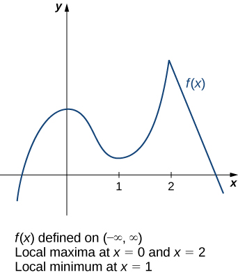
Consider the function \(f\) shown in Figure \(\PageIndex{3}\). The graph can be described as two mountains with a valley in the middle. The absolute maximum value of the function occurs at the higher peak, at \(x=2\). However, \(x=0\) is also a point of interest. Although \(f(0)\) is not the largest value of \(f\), the value \(f(0)\) is larger than \(f(x)\) for all \(x\) near 0. We say \(f\) has a local maximum at \(x=0\). Similarly, the function \(f\) does not have an absolute minimum, but it does have a local minimum at \(x=1\) because \(f(1)\) is less than \(f(x)\) for \(x\) near 1.

Figure \(\PageIndex{3}\): This function \(f\) has two local maxima and one local minimum. The local maximum at \(x=2\) is also the absolute maximum.

Definition: Local Extrema

A function \(f\) has a local maximum at \(c\) if there exists an open interval \(I\) containing \(c\) such that \(I\) is contained in the domain of \(f\) and \(f(c)≥f(x)\) for all \(x∈I\). A function \(f\) has a local minimum at \(c\) if there exists an open interval \(I\) containing \(c\) such that \(I\) is contained in the domain of \(f\) and \(f(c)≤f(x)\) for all \(x∈I\). A function \(f\) has a local extremum at \(c\) if \(f\) has a local maximum at \(c\) or \(f\) has a local minimum at \(c\).

Note that if \(f\) has an absolute extremum at \(c\) and \(f\) is defined over an interval containing \(c\), then \(f(c)\) is also considered a local extremum. If an absolute extremum for a function \(f\) occurs at an endpoint, we do not consider that to be a local extremum, but instead refer to that as an endpoint extremum.

Given the graph of a function \(f\), it is sometimes easy to see where a local maximum or local minimum occurs. However, it is not always easy to see, since the interesting features on the graph of a function may not be visible because they occur at a very small scale. Also, we may not have a graph of the function. In these cases, how can we use a formula for a function to determine where these extrema occur?

To answer this question, let’s look at Figure \(\PageIndex{3}\) again. The local extrema occur at \(x=0, x=1,\) and \(x=2.\) Notice that at \(x=0\) and \(x=1\), the derivative \(f'(x)=0\). At \(x=2\), the derivative \(f'(x)\) does not exist, since the function \(f\) has a corner there. In fact, if \(f\) has a local extremum at a point \(x=c\), the derivative \(f'(c)\) must satisfy one of the following conditions: either \(f'(c)=0\) or \(f'(c)\) is undefined. Such a value \(c\) is known as a critical point and it is important in finding extreme values for functions.

Definition: Critical Points

Let \(c\) be an interior point in the domain of \(f\). We say that \(c\) is a critical point of \(f\) if \(f'(c)=0\) or \(f'(c)\) is undefined.

As mentioned earlier, if \(f\) has a local extremum at a point \(x=c\), then \(c\) must be a critical point of \(f\). This fact is known as Fermat’s theorem.

Theorem \(\PageIndex{2}\): Fermat’s Theorem

If \(f\) has a local extremum at \(c\) and \(f\) is differentiable at \(c\), then \(f'(c)=0.\)

Proof

Suppose \(f\) has a local extremum at \(c\) and \(f\) is differentiable at \(c\). We need to show that \(f'(c)=0\). To do this, we will show that \(f'(c)≥0\) and \(f'(c)≤0\), and therefore \(f'(c)=0\). Since \(f\) has a local extremum at \(c\), \(f\) has a local maximum or local minimum at \(c\). Suppose \(f\) has a local maximum at \(c\). The case in which \(f\) has a local minimum at \(c\) can be handled similarly. There then exists an open interval I such that \(f(c)≥f(x)\) for all \(x∈I\). Since \(f\) is differentiable at \(c\), from the definition of the derivative, we know that

\[f'(c)=\lim_{x→c}\frac{f(x)−f(c)}{x−c}. \nonumber \]

Since this limit exists, both one-sided limits also exist and equal \(f'(c)\). Therefore,

\[f'(c)=\lim_{x→c^+}\frac{f(x)−f(c)}{x−c,}\label{FermatEqn2} \]

and

\[f'(c)=\lim_{x→c^−}\frac{f(x)−f(c)}{x−c}. \nonumber \]

Since \(f(c)\) is a local maximum, we see that \(f(x)−f(c)≤0\) for \(x\) near \(c\). Therefore, for \(x\) near \(c\), but \(x>c\), we have \(\frac{f(x)−f(c)}{x−c}≤0\). From Equation \ref{FermatEqn2} we conclude that \(f'(c)≤0\). Similarly, it can be shown that \(f'(c)≥0.\) Therefore, \(f'(c)=0.\)

□

From Fermat’s theorem, we conclude that if \(f\) has a local extremum at \(c\), then either \(f'(c)=0\) or \(f'(c)\) is undefined. In other words, local extrema can only occur at critical points.

Note this theorem does not claim that a function \(f\) must have a local extremum at a critical point. Rather, it states that critical points are candidates for local extrema. For example, consider the function \(f(x)=x^3\). We have \(f'(x)=3x^2=0\) when \(x=0\). Therefore, \(x=0\) is a critical point. However, \(f(x)=x^3\) is increasing over \((−∞,∞)\), and thus \(f\) does not have a local extremum at \(x=0\). In Figure \(\PageIndex{4}\), we see several different possibilities for critical points. In some of these cases, the functions have local extrema at critical points, whereas in other cases the functions do not. Note that these graphs do not show all possibilities for the behavior of a function at a critical point.

Figure \(\PageIndex{4}\): (a–e) A function \(f\) has a critical point at \(c\) if \(f'(c)=0\) or \(f'(c)\) is undefined. A function may or may not have a local extremum at a critical point.

Later in this chapter we look at analytical methods for determining whether a function actually has a local extremum at a critical point. For now, let’s turn our attention to finding critical points. We will use graphical observations to determine whether a critical point is associated with a local extremum.

Example \(\PageIndex{1}\): Locating Critical Points

For each of the following functions, find all critical points. Use a graphing utility to determine whether the function has a local extremum at each of the critical points.

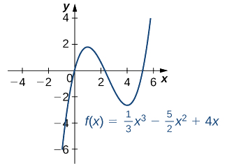
1. \(f(x)=\frac{1}{3}x^3−\frac{5}{2}x^2+4x\)
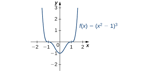
2. \(f(x)=(x^2−1)^3\)
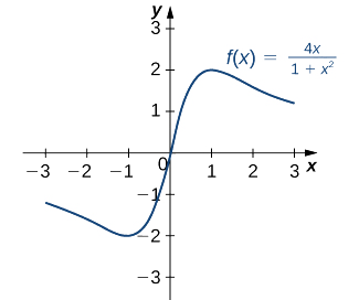
3. \(f(x)=\frac{4x}{1+x^2}\)

Solution

a. The derivative \(f'(x)=x^2−5x+4\) is defined for all real numbers \(x\). Therefore, we only need to find the values for \(x\) where \(f'(x)=0\). Since \(f'(x)=x^2−5x+4=(x−4)(x−1)\), the critical points are \(x=1\) and \(x=4.\) From the graph of \(f\) in Figure \(\PageIndex{5}\), we see that \(f\) has a local maximum at \(x=1\) and a local minimum at \(x=4\).

Figure \(\PageIndex{5}\): This function has a local maximum and a local minimum.

b. Using the chain rule, we see the derivative is

\(f'(x)=3(x^2−1)^2(2x)=6x(x^2−1)^2.\)

Therefore, \(f\) has critical points when \(x=0\) and when \(x^2−1=0\). We conclude that the critical points are \(x=0,±1\). From the graph of \(f\) in Figure \(\PageIndex{6}\), we see that \(f\) has a local (and absolute) minimum at \(x=0\), but does not have a local extremum at \(x=1\) or \(x=−1\).

Figure \(\PageIndex{6}\): This function has three critical points: \(x=0\), \(x=1\), and \(x=−1\). The function has a local (and absolute) minimum at \(x=0\), but does not have extrema at the other two critical points.

c. By the quotient rule, we see that the derivative is

\(f'(x)=\frac{4(1+x^2)−4x(2x)}{(1+x^2)^2}=\frac{4−4x^2}{(1+x^2)^2}\).

The derivative is defined everywhere. Therefore, we only need to find values for \(x\) where \(f'(x)=0\). Solving \(f'(x)=0\), we see that \(4−4x^2=0,\) which implies \(x=±1\). Therefore, the critical points are \(x=±1\). From the graph of \(f\) in Figure \(\PageIndex{7}\), we see that f has an absolute maximum at \(x=1\) and an absolute minimum at \(x=−1.\) Hence, \(f\) has a local maximum at \(x=1\) and a local minimum at \(x=−1\). (Note that if \(f\) has an absolute extremum over an interval \(I\) at a point \(c\) that is not an endpoint of \(I\), then \(f\) has a local extremum at \(c.)\)

Figure \(\PageIndex{7}\): This function has an absolute maximum and an absolute minimum.

Exercise \(\PageIndex{1}\)

Find all critical points for \(f(x)=x^3−\frac{1}{2}x^2−2x+1.\)

Hint

Calculate \(f'(x).\)

Answer

\(x=\frac{−2}{3}, x=1\)

Locating Absolute Extrema

The extreme value theorem states that a continuous function over a closed, bounded interval has an absolute maximum and an absolute minimum. As shown in Figure \(\PageIndex{2}\), one or both of these absolute extrema could occur at an endpoint. If an absolute extremum does not occur at an endpoint, however, it must occur at an interior point, in which case the absolute extremum is a local extremum. Therefore, by Fermat's Theorem, the point \(c\) at which the local extremum occurs must be a critical point. We summarize this result in the following theorem.

Theorem \(\PageIndex{3}\): Location of Absolute Extrema

Let \(f\) be a continuous function over a closed, bounded interval \(I\). The absolute maximum of \(f\) over \(I\) and the absolute minimum of \(f\) over \(I\) must occur at endpoints of \(I\) or at critical points of \(f\) in \(I\).

With this idea in mind, let’s examine a procedure for locating absolute extrema.

Problem-Solving Strategy: Locating Absolute Extrema over a Closed Interval

Consider a continuous function \(f\) defined over the closed interval \([a,b].\)

1. Evaluate \(f\) at the endpoints \(x=a\) and \(x=b.\)
2. Find all critical points of \(f\) that lie over the interval \((a,b)\) and evaluate \(f\) at those critical points.
3. Compare all values found in (1) and (2). From "Location of Absolute Extrema," the absolute extrema must occur at endpoints or critical points. Therefore, the largest of these values is the absolute maximum of \(f\). The smallest of these values is the absolute minimum of \(f\).

Now let’s look at how to use this strategy to find the absolute maximum and absolute minimum values for continuous functions.

Example \(\PageIndex{2}\): Locating Absolute Extrema

For each of the following functions, find the absolute maximum and absolute minimum over the specified interval and state where those values occur.

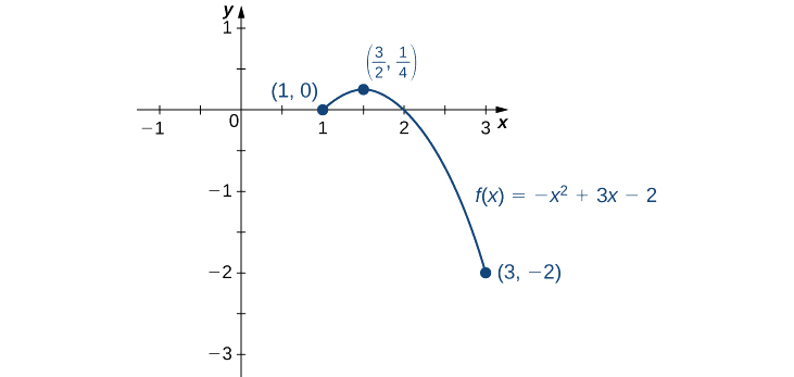
1. \(f(x)=−x^2+3x−2\) over \([1,3].\)
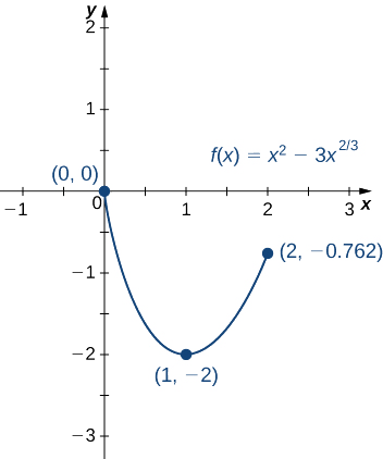
2. \(f(x)=x^2−3x^{2/3}\) over \([0,2]\).

Solution

a. Step 1. Evaluate \(f\) at the endpoints \(x=1\) and \(x=3\).

\(f(1)=0\) and \(f(3)=−2\)

Step 2. Since \(f'(x)=−2x+3, f'\) is defined for all real numbers \(x.\) Therefore, there are no critical points where the derivative is undefined. It remains to check where \(f'(x)=0\). Since \(f'(x)=−2x+3=0 \) at \(x=\frac{3}{2}\) and \(\frac{3}{2}\) is in the interval \([1,3], f(\frac{3}{2})\) is a candidate for an absolute extremum of \(f\) over \([1,3]\). We evaluate \(f(\frac{3}{2})\) and find

\(f\left(\frac{3}{2}\right)=\frac{1}{4}\).

Step 3. We set up the following table to compare the values found in steps 1 and 2.

\(x\)	\(f(x)\)	Conclusion
\(1\)	\(0\)
\(\frac{3}{2}\)	\(\frac{1}{4}\)	Absolute maximum
\(3\)	\(−2\)	Absolute minimum

From the table, we find that the absolute maximum of \(f\) over the interval [1, 3] is \(\frac{1}{4}\), and it occurs at \(x=\frac{3}{2}\). The absolute minimum of \(f\) over the interval \([1, 3]\) is \(−2\), and it occurs at \(x=3\) as shown in Figure \(\PageIndex{8}\).

Figure \(\PageIndex{8}\): This function has both an absolute maximum and an absolute minimum.

b. Step 1. Evaluate \(f\) at the endpoints \(x=0\) and \(x=2\).

\(f(0)=0\) and \(f(2)=4−3\left(2\right)^{2/3}≈−0.762\)

Step 2. The derivative of \(f\) is given by

\(f'(x)=2x−\frac{2}{x^{1/3}}=\dfrac{2x^{4/3}−2}{x^{1/3}}\)

for \(x≠0\). The derivative is zero when \(2x^{4/3}−2=0\), which implies \(x=±1\). The derivative is undefined at \(x=0\). Therefore, the critical points of \(f\) are \(x=0,1,−1\). The point \(x=0\) is an endpoint, so we already evaluated \(f(0)\) in step 1. The point \(x=−1\) is not in the interval of interest, so we need only evaluate \(f(1)\). We find that

\(f(1)=−2.\)

Step 3. We compare the values found in steps 1 and 2, in the following table.

\(x\)	\(f(x)\)	Conclusion
\(0\)	\(0\)	Absolute maximum
\(1\)	\(−2\)	Absolute minimum
\(2\)	\(−0.762\)

We conclude that the absolute maximum of \(f\) over the interval \([0, 2]\) is zero, and it occurs at \(x=0\). The absolute minimum is \(−2,\) and it occurs at \(x=1\) as shown in Figure \(\PageIndex{9}\).

Figure \(\PageIndex{9}\): This function has an absolute maximum at an endpoint of the interval.

Exercise \(\PageIndex{2}\)

Find the absolute maximum and absolute minimum of \(f(x)=x^2−4x+3\) over the interval \([1,4]\).

Hint

Look for critical points. Evaluate \(f\) at all critical points and at the endpoints.

Answer

The absolute maximum is \(3\) and it occurs at \(x=4\). The absolute minimum is \(−1\) and it occurs at \(x=2\).

At this point, we know how to locate absolute extrema for continuous functions over closed intervals. We have also defined local extrema and determined that if a function \(f\) has a local extremum at a point \(c\), then \(c\) must be a critical point of \(f\). However, \(c\) being a critical point is not a sufficient condition for \(f\) to have a local extremum at \(c\). Later in this chapter, we show how to determine whether a function actually has a local extremum at a critical point. First, however, we need to introduce the Mean Value Theorem, which will help as we analyze the behavior of the graph of a function.

Solving Optimization Problems over a Closed, Bounded Interval

The basic idea of the optimization problems that follow is the same. We have a particular quantity that we are interested in maximizing or minimizing. However, we also have some auxiliary condition that needs to be satisfied. For example, in Example \(\PageIndex{1}\), we are interested in maximizing the area of a rectangular garden. Certainly, if we keep making the side lengths of the garden larger, the area will continue to become larger. However, what if we have some restriction on how much fencing we can use for the perimeter? In this case, we cannot make the garden as large as we like. Let’s look at how we can maximize the area of a rectangle subject to some constraint on the perimeter.

Example \(\PageIndex{1}\): Maximizing the Area of a Garden

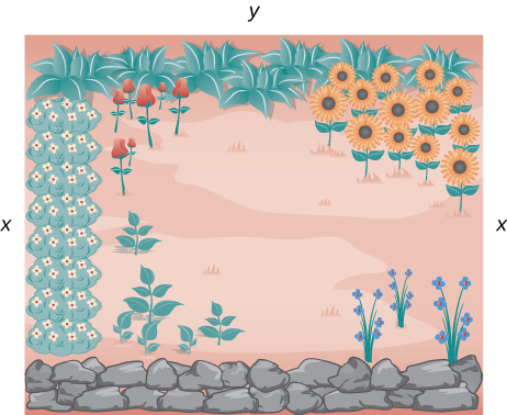
A rectangular garden is to be constructed using a rock wall as one side of the garden and wire fencing for the other three sides (Figure \(\PageIndex{1}\)). Given \(100\,\text{ft}\) of wire fencing, determine the dimensions that would create a garden of maximum area. What is the maximum area?

Figure \(\PageIndex{1}\): We want to determine the measurements \(x\) and \(y\) that will create a garden with a maximum area using \(100\,\text{ft}\) of fencing.

Solution

Let \(x\) denote the length of the side of the garden perpendicular to the rock wall and \(y\) denote the length of the side parallel to the rock wall. Then the area of the garden is

\(A=x⋅y.\)

We want to find the maximum possible area subject to the constraint that the total fencing is \(100\,\text{ft}\). From Figure \(\PageIndex{1}\), the total amount of fencing used will be \(2x+y.\) Therefore, the constraint equation is

\(2x+y=100.\)

Solving this equation for \(y\), we have \(y=100−2x.\) Thus, we can write the area as

\(A(x)=x⋅(100−2x)=100x−2x^2.\)

Before trying to maximize the area function \(A(x)=100x−2x^2,\) we need to determine the domain under consideration. To construct a rectangular garden, we certainly need the lengths of both sides to be positive. Therefore, we need \(x>0\) and \(y>0\). Since \(y=100−2x\), if \(y>0\), then \(x<50\). Therefore, we are trying to determine the maximum value of \(A(x)\) for \(x\) over the open interval \((0,50)\). We do not know that a function necessarily has a maximum value over an open interval. However, we do know that a continuous function has an absolute maximum (and absolute minimum) over a closed interval. Therefore, let’s consider the function \(A(x)=100x−2x^2\) over the closed interval \([0,50]\). If the maximum value occurs at an interior point, then we have found the value \(x\) in the open interval \((0,50)\) that maximizes the area of the garden.

Therefore, we consider the following problem:

Maximize \(A(x)=100x−2x^2\) over the interval \([0,50].\)

As mentioned earlier, since \(A\) is a continuous function on a closed, bounded interval, by the extreme value theorem, it has a maximum and a minimum. These extreme values occur either at endpoints or critical points. At the endpoints, \(A(x)=0\). Since the area is positive for all \(x\) in the open interval \((0,50)\), the maximum must occur at a critical point. Differentiating the function \(A(x)\), we obtain

\(A′(x)=100−4x.\)

Therefore, the only critical point is \(x=25\) (Figure \(\PageIndex{2}\)). We conclude that the maximum area must occur when \(x=25\).

Figure \(\PageIndex{2}\): To maximize the area of the garden, we need to find the maximum value of the function \(A(x)=100x−2x^2\).

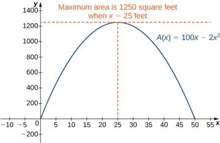
Then we have \(y=100−2x=100−2(25)=50.\) To maximize the area of the garden, let \(x=25\,\text{ft}\) and \(y=50\,\text{ft}\). The area of this garden is \(1250\, \text{ft}^2\).

Exercise \(\PageIndex{1}\)

Determine the maximum area if we want to make the same rectangular garden as in Figure \(\PageIndex{2}\), but we have \(200\,\text{ft}\) of fencing.

Hint

We need to maximize the function \(A(x)=200x−2x^2\) over the interval \([0,100].\)

Answer

The maximum area is \(5000\, \text{ft}^2\).

Now let’s look at a general strategy for solving optimization problems similar to Example \(\PageIndex{1}\).

Problem-Solving Strategy: Solving Optimization Problems

1. Introduce all variables. If applicable, draw a figure and label all variables.
2. Determine which quantity is to be maximized or minimized, and for what range of values of the other variables (if this can be determined at this time).
3. Write a formula for the quantity to be maximized or minimized in terms of the variables. This formula may involve more than one variable.
4. Write any equations relating the independent variables in the formula from step \(3\). Use these equations to write the quantity to be maximized or minimized as a function of one variable.
5. Identify the domain of consideration for the function in step \(4\) based on the physical problem to be solved.
6. Locate the maximum or minimum value of the function from step \(4.\) This step typically involves looking for critical points and evaluating a function at endpoints.

Now let’s apply this strategy to maximize the volume of an open-top box given a constraint on the amount of material to be used.

Example \(\PageIndex{2}\): Maximizing the Volume of a Box

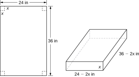
An open-top box is to be made from a \(24\,\text{in.}\) by \(36\,\text{in.}\) piece of cardboard by removing a square from each corner of the box and folding up the flaps on each side. What size square should be cut out of each corner to get a box with the maximum volume?

Solution

Step 1: Let \(x\) be the side length of the square to be removed from each corner (Figure \(\PageIndex{3}\)). Then, the remaining four flaps can be folded up to form an open-top box. Let \(V\) be the volume of the resulting box.

Figure \(\PageIndex{3}\): A square with side length \(x\) inches is removed from each corner of the piece of cardboard. The remaining flaps are folded to form an open-top box.

Step 2: We are trying to maximize the volume of a box. Therefore, the problem is to maximize \(V\).

Step 3: As mentioned in step 2, are trying to maximize the volume of a box. The volume of a box is

\[V=L⋅W⋅H \nonumber, \nonumber \]

where \(L,\,W,\)and \(H\) are the length, width, and height, respectively.

Step 4: From Figure \(\PageIndex{3}\), we see that the height of the box is \(x\) inches, the length is \(36−2x\) inches, and the width is \(24−2x\) inches. Therefore, the volume of the box is

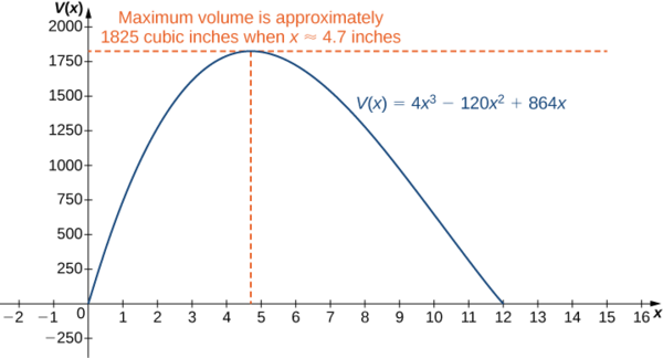
\[ \begin{align*} V(x) &=(36−2x)(24−2x)x \\[4pt] &=4x^3−120x^2+864x \end{align*}. \nonumber \]

Step 5: To determine the domain of consideration, let’s examine Figure \(\PageIndex{3}\). Certainly, we need \(x>0.\) Furthermore, the side length of the square cannot be greater than or equal to half the length of the shorter side, \(24\,\text{in.}\); otherwise, one of the flaps would be completely cut off. Therefore, we are trying to determine whether there is a maximum volume of the box for \(x\) over the open interval \((0,12).\) Since \(V\) is a continuous function over the closed interval \([0,12]\), we know \(V\) will have an absolute maximum over the closed interval. Therefore, we consider \(V\) over the closed interval \([0,12]\) and check whether the absolute maximum occurs at an interior point.

Step 6: Since \(V(x)\) is a continuous function over the closed, bounded interval \([0,12]\), \(V\) must have an absolute maximum (and an absolute minimum). Since \(V(x)=0\) at the endpoints and \(V(x)>0\) for \(0<x<12,\) the maximum must occur at a critical point. The derivative is

\(V′(x)=12x^2−240x+864.\)

To find the critical points, we need to solve the equation

\(12x^2−240x+864=0.\)

Dividing both sides of this equation by \(12\), the problem simplifies to solving the equation

\(x^2−20x+72=0.\)

Using the quadratic formula, we find that the critical points are

\[\begin{align*} x &=\dfrac{20±\sqrt{(−20)^2−4(1)(72)}}{2} \\[4pt] &=\dfrac{20±\sqrt{112}}{2} \\[4pt] &=\dfrac{20±4\sqrt{7}}{2} \\[4pt] &=10±2\sqrt{7} \end{align*}. \nonumber \]

Since \(10+2\sqrt{7}\) is not in the domain of consideration, the only critical point we need to consider is \(10−2\sqrt{7}\). Therefore, the volume is maximized if we let \(x=10−2\sqrt{7}\,\text{in.}\) The maximum volume is

\[V(10−2\sqrt{7})=640+448\sqrt{7}≈1825\,\text{in}^3. \nonumber \]

as shown in the following graph.

Figure \(\PageIndex{4}\): Maximizing the volume of the box leads to finding the maximum value of a cubic polynomial.

Exercise \(\PageIndex{2}\)

Suppose the dimensions of the cardboard in Example \(\PageIndex{2}\) are \(20\,\text{in.}\) by \(30\,\text{in.}\) Let \(x\) be the side length of each square and write the volume of the open-top box as a function of \(x\). Determine the domain of consideration for \(x\).

Hint

The volume of the box is \(L⋅W⋅H.\)

Answer

\(V(x)=x(20−2x)(30−2x).\) The domain is \([0,10]\).

Example \(\PageIndex{3}\): Minimizing Travel Time

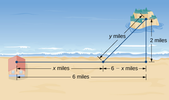
An island is \(2\) mi due north of its closest point along a straight shoreline. A visitor is staying at a cabin on the shore that is \(6\) mi west of that point. The visitor is planning to go from the cabin to the island. Suppose the visitor runs at a rate of \(8\) mph and swims at a rate of \(3\) mph. How far should the visitor run before swimming to minimize the time it takes to reach the island?

Solution

Step 1: Let \(x\) be the distance running and let \(y\) be the distance swimming (Figure \(\PageIndex{5}\)). Let \(T\) be the time it takes to get from the cabin to the island.

Figure \(\PageIndex{5}\): How can we choose \(x\) and \(y\) to minimize the travel time from the cabin to the island?

Step 2: The problem is to minimize \(T\).

Step 3: To find the time spent traveling from the cabin to the island, add the time spent running and the time spent swimming. Since Distance = Rate × Time \((D=R×T),\) the time spent running is

\(T_{running}=\dfrac{D_{running}}{R_{running}}=\dfrac{x}{8}\),

and the time spent swimming is

\(T_{swimming}=\dfrac{D_{swimming}}{R_{swimming}}=\dfrac{y}{3}\).

Therefore, the total time spent traveling is

\(T=\dfrac{x}{8}+\dfrac{y}{3}\).

Step 4: From Figure \(\PageIndex{5}\), the line segment of \(y\) miles forms the hypotenuse of a right triangle with legs of length \(2\) mi and \(6−x\) mi. Therefore, by the Pythagorean theorem, \(2^2+(6−x)^2=y^2\), and we obtain \(y=\sqrt{(6−x)^2+4}\). Thus, the total time spent traveling is given by the function

\(T(x)=\dfrac{x}{8}+\dfrac{\sqrt{(6−x)^2+4}}{3}\).

Step 5: From Figure \(\PageIndex{5}\), we see that \(0≤x≤6\). Therefore, \([0,6]\) is the domain of consideration.

Step 6: Since \(T(x)\) is a continuous function over a closed, bounded interval, it has a maximum and a minimum. Let’s begin by looking for any critical points of \(T\) over the interval \([0,6].\) The derivative is

\[\begin{align*} T′(x) &=\dfrac{1}{8}−\dfrac{1}{2}\dfrac{[(6−x)^2+4]^{−1/2}}{3}⋅2(6−x) \\[4pt] &=\dfrac{1}{8}−\dfrac{(6−x)}{3\sqrt{(6−x)^2+4}} \end{align*}\]

If \(T′(x)=0,\), then

\[\dfrac{1}{8}=\dfrac{6−x}{3\sqrt{(6−x)^2+4}} \label{ex3eq1} \]

Therefore,

\[3\sqrt{(6−x)^2+4}=8(6−x). \label{ex3eq2} \]

Squaring both sides of this equation, we see that if \(x\) satisfies this equation, then \(x\) must satisfy

\[9[(6−x)^2+4]=64(6−x)^2,\nonumber \]

which implies

\[55(6−x)^2=36. \nonumber \]

We conclude that if \(x\) is a critical point, then \(x\) satisfies

\[(x−6)^2=\dfrac{36}{55}. \nonumber \]

[Note that since we are squaring, \( (x-6)^2 = (6-x)^2.\)]

Therefore, the possibilities for critical points are

\[x=6±\dfrac{6}{\sqrt{55}}.\nonumber \]

Since \(x=6+6/\sqrt{55}\) is not in the domain, it is not a possibility for a critical point. On the other hand, \(x=6−6/\sqrt{55}\) is in the domain. Since we squared both sides of Equation \ref{ex3eq2} to arrive at the possible critical points, it remains to verify that \(x=6−6/\sqrt{55}\) satisfies Equation \ref{ex3eq1}. Since \(x=6−6/\sqrt{55}\) does satisfy that equation, we conclude that \(x=6−6/\sqrt{55}\) is a critical point, and it is the only one. To justify that the time is minimized for this value of \(x\), we just need to check the values of \(T(x)\) at the endpoints \(x=0\) and \(x=6\), and compare them with the value of \(T(x)\) at the critical point \(x=6−6/\sqrt{55}\). We find that \(T(0)≈2.108\,\text{h}\) and \(T(6)≈1.417\,\text{h}\), whereas

\[T(6−6/\sqrt{55})≈1.368\,\text{h}. \nonumber \]

Therefore, we conclude that \(T\) has a local minimum at \(x≈5.19\) mi.

Exercise \(\PageIndex{3}\)

Suppose the island is \(1\) mi from shore, and the distance from the cabin to the point on the shore closest to the island is \(15\) mi. Suppose a visitor swims at the rate of \(2.5\) mph and runs at a rate of \(6\) mph. Let \(x\) denote the distance the visitor will run before swimming, and find a function for the time it takes the visitor to get from the cabin to the island.

Hint

The time \(T=T_{running}+T_{swimming}.\)

Answer

\(T(x)=\dfrac{x}{6}+\dfrac{\sqrt{(15−x)^2+1}}{2.5} \)

In business, companies are interested in maximizing revenue. In the following example, we consider a scenario in which a company has collected data on how many cars it is able to lease, depending on the price it charges its customers to rent a car. Let’s use these data to determine the price the company should charge to maximize the amount of money it brings in.

Example \(\PageIndex{4}\): Maximizing Revenue

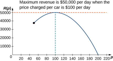
Owners of a car rental company have determined that if they charge customers \(p\) dollars per day to rent a car, where \(50≤p≤200\), the number of cars \(n\) they rent per day can be modeled by the linear function \(n(p)=1000−5p\). If they charge \($50\) per day or less, they will rent all their cars. If they charge \($200\) per day or more, they will not rent any cars. Assuming the owners plan to charge customers between \($50\) per day and \($200\) per day to rent a car, how much should they charge to maximize their revenue?

Solution

Step 1: Let \(p\) be the price charged per car per day and let \(n\) be the number of cars rented per day. Let \(R\) be the revenue per day.

Step 2: The problem is to maximize \(R.\)

Step 3: The revenue (per day) is equal to the number of cars rented per day times the price charged per car per day—that is, \(R=n×p.\)

Step 4: Since the number of cars rented per day is modeled by the linear function \(n(p)=1000−5p,\) the revenue \(R\) can be represented by the function

\[ \begin{align*} R(p) &=n×p \\[4pt] &=(1000−5p)p \\[4pt] &=−5p^2+1000p.\end{align*}\]

Step 5: Since the owners plan to charge between \($50\) per car per day and \($200\) per car per day, the problem is to find the maximum revenue \(R(p)\) for \(p\) in the closed interval \([50,200]\).

Step 6: Since \(R\) is a continuous function over the closed, bounded interval \([50,200]\), it has an absolute maximum (and an absolute minimum) in that interval. To find the maximum value, look for critical points. The derivative is \(R′(p)=−10p+1000.\) Therefore, the critical point is \(p=100\). When \(p=100, R(100)=$50,000.\) When \(p=50, R(p)=$37,500\). When \(p=200, R(p)=$0\).

Therefore, the absolute maximum occurs at \(p=$100\). The car rental company should charge \($100\) per day per car to maximize revenue as shown in the following figure.

Figure \(\PageIndex{6}\): To maximize revenue, a car rental company has to balance the price of a rental against the number of cars people will rent at that price.

Exercise \(\PageIndex{4}\)

A car rental company charges its customers \(p\) dollars per day, where \(60≤p≤150\). It has found that the number of cars rented per day can be modeled by the linear function \(n(p)=750−5p.\) How much should the company charge each customer to maximize revenue?

Hint

\(R(p)=n×p,\) where \(n\) is the number of cars rented and \(p\) is the price charged per car.

Answer

The company should charge \($75\) per car per day.

Example \(\PageIndex{5}\): Maximizing the Area of an Inscribed Rectangle

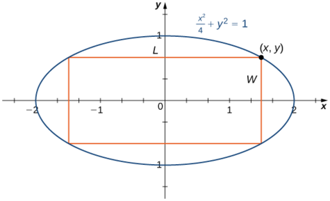
A rectangle is to be inscribed in the ellipse

\[\dfrac{x^2}{4}+y^2=1. \nonumber \]

What should the dimensions of the rectangle be to maximize its area? What is the maximum area?

Solution

Step 1: For a rectangle to be inscribed in the ellipse, the sides of the rectangle must be parallel to the axes. Let \(L\) be the length of the rectangle and \(W\) be its width. Let \(A\) be the area of the rectangle.

Figure \(\PageIndex{7}\): We want to maximize the area of a rectangle inscribed in an ellipse.

Step 2: The problem is to maximize \(A\).

Step 3: The area of the rectangle is \(A=LW.\)

Step 4: Let \((x,y)\) be the corner of the rectangle that lies in the first quadrant, as shown in Figure \(\PageIndex{7}\). We can write length \(L=2x\) and width \(W=2y\). Since \(\dfrac{x^2}{4}+y^2=1\) and \(y>0\), we have \(y=\sqrt{1-\dfrac{x^2}{4}}\). Therefore, the area is

\(A=LW=(2x)(2y)=4x\sqrt{1-\dfrac{x^2}{4}}=2x\sqrt{4−x^2}\)

Step 5: From Figure \(\PageIndex{7}\), we see that to inscribe a rectangle in the ellipse, the \(x\)-coordinate of the corner in the first quadrant must satisfy \(0<x<2\). Therefore, the problem reduces to looking for the maximum value of \(A(x)\) over the open interval \((0,2)\). Since \(A(x)\) will have an absolute maximum (and absolute minimum) over the closed interval \([0,2]\), we consider \(A(x)=2x\sqrt{4−x^2}\) over the interval \([0,2]\). If the absolute maximum occurs at an interior point, then we have found an absolute maximum in the open interval.

Step 6: As mentioned earlier, \(A(x)\) is a continuous function over the closed, bounded interval \([0,2]\). Therefore, it has an absolute maximum (and absolute minimum). At the endpoints \(x=0\) and \(x=2\), \(A(x)=0.\) For \(0<x<2\), \(A(x)>0\).

Therefore, the maximum must occur at a critical point. Taking the derivative of \(A(x)\), we obtain

\[ \begin{align*} A'(x) &=2\sqrt{4−x^2}+2x⋅\dfrac{1}{2\sqrt{4−x^2}}(−2x) \\[4pt] &=2\sqrt{4−x^2}−\dfrac{2x^2}{\sqrt{4−x^2}} \\[4pt] &=\dfrac{8−4x^2}{\sqrt{4−x^2}} . \end{align*}\]

To find critical points, we need to find where \(A'(x)=0.\) We can see that if \(x\) is a solution of

\[\dfrac{8−4x^2}{\sqrt{4−x^2}}=0, \label{ex5eq1} \]

then \(x\) must satisfy

\[8−4x^2=0. \nonumber \]

Therefore, \(x^2=2.\) Thus, \(x=±\sqrt{2}\) are the possible solutions of Equation \ref{ex5eq1}. Since we are considering \(x\) over the interval \([0,2]\), \(x=\sqrt{2}\) is a possibility for a critical point, but \(x=−\sqrt{2}\) is not. Therefore, we check whether \(\sqrt{2}\) is a solution of Equation \ref{ex5eq1}. Since \(x=\sqrt{2}\) is a solution of Equation \ref{ex5eq1}, we conclude that \(\sqrt{2}\) is the only critical point of \(A(x)\) in the interval \([0,2]\).

Therefore, \(A(x)\) must have an absolute maximum at the critical point \(x=\sqrt{2}\). To determine the dimensions of the rectangle, we need to find the length \(L\) and the width \(W\). If \(x=\sqrt{2}\) then

\[y=\sqrt{1−\dfrac{(\sqrt{2})^2}{4}}=\sqrt{1−\dfrac{1}{2}}=\dfrac{1}{\sqrt{2}}.\nonumber \]

Therefore, the dimensions of the rectangle are \(L=2x=2\sqrt{2}\) and \(W=2y=\dfrac{2}{\sqrt{2}}=\sqrt{2}\). The area of this rectangle is \( A=LW=(2\sqrt{2})(\sqrt{2})=4.\)

Exercise \(\PageIndex{5}\)

Modify the area function \(A\) if the rectangle is to be inscribed in the unit circle \(x^2+y^2=1\). What is the domain of consideration?

Hint

If \((x,y)\) is the vertex of the square that lies in the first quadrant, then the area of the square is \(A=(2x)(2y)=4xy.\)

Answer

\(A(x)=4x\sqrt{1−x^2}.\) The domain of consideration is \([0,1]\).

Solving Optimization Problems when the Interval Is Not Closed or Is Unbounded

In the previous examples, we considered functions on closed, bounded domains. Consequently, by the extreme value theorem, we were guaranteed that the functions had absolute extrema. Let’s now consider functions for which the domain is neither closed nor bounded.

Many functions still have at least one absolute extrema, even if the domain is not closed or the domain is unbounded. For example, the function \(f(x)=x^2+4\) over \((−∞,∞)\) has an absolute minimum of \(4\) at \(x=0\). Therefore, we can still consider functions over unbounded domains or open intervals and determine whether they have any absolute extrema. In the next example, we try to minimize a function over an unbounded domain. We will see that, although the domain of consideration is \((0,∞),\) the function has an absolute minimum.

In the following example, we look at constructing a box of least surface area with a prescribed volume. It is not difficult to show that for a closed-top box, by symmetry, among all boxes with a specified volume, a cube will have the smallest surface area. Consequently, we consider the modified problem of determining which open-topped box with a specified volume has the smallest surface area.

Example \(\PageIndex{6}\): Minimizing Surface Area

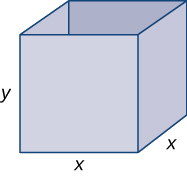
A rectangular box with a square base, an open top, and a volume of \(216 \,\text{in}^3\) is to be constructed. What should the dimensions of the box be to minimize the surface area of the box? What is the minimum surface area?

Solution

Step 1: Draw a rectangular box and introduce the variable \(x\) to represent the length of each side of the square base; let \(y\) represent the height of the box. Let \(S\) denote the surface area of the open-top box.

Figure \(\PageIndex{8}\): We want to minimize the surface area of a square-based box with a given volume.

Step 2: We need to minimize the surface area. Therefore, we need to minimize \(S\).

Step 3: Since the box has an open top, we need only determine the area of the four vertical sides and the base. The area of each of the four vertical sides is \(x⋅y.\) The area of the base is \(x^2\). Therefore, the surface area of the box is

\(S=4xy+x^2\).

Step 4: Since the volume of this box is \(x^2y\) and the volume is given as \(216\,\text{in}^3\), the constraint equation is

\(x^2y=216\).

Solving the constraint equation for \(y\), we have \(y=\dfrac{216}{x^2}\). Therefore, we can write the surface area as a function of \(x\) only:

\[S(x)=4x\left(\dfrac{216}{x^2}\right)+x^2.\nonumber \]

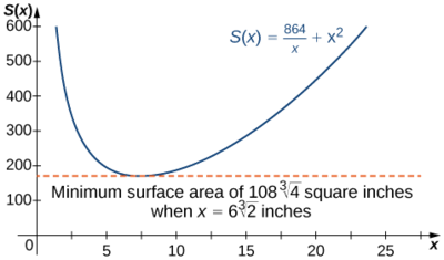
Therefore, \(S(x)=\dfrac{864}{x}+x^2\).

Step 5: Since we are requiring that \(x^2y=216\), we cannot have \(x=0\). Therefore, we need \(x>0\). On the other hand, \(x\) is allowed to have any positive value. Note that as \(x\) becomes large, the height of the box \(y\) becomes correspondingly small so that \(x^2y=216\). Similarly, as \(x\) becomes small, the height of the box becomes correspondingly large. We conclude that the domain is the open, unbounded interval \((0,∞)\). Note that, unlike the previous examples, we cannot reduce our problem to looking for an absolute maximum or absolute minimum over a closed, bounded interval. However, in the next step, we discover why this function must have an absolute minimum over the interval \((0,∞).\)

Step 6: Note that as \(x→0^+,\, S(x)→∞.\) Also, as \(x→∞, \,S(x)→∞\). Since \(S\) is a continuous function that approaches infinity at the ends, it must have an absolute minimum at some \(x∈(0,∞)\). This minimum must occur at a critical point of \(S\). The derivative is

\[S′(x)=−\dfrac{864}{x^2}+2x.\nonumber \]

Therefore, \(S′(x)=0\) when \(2x=\dfrac{864}{x^2}\). Solving this equation for \(x\), we obtain \(x^3=432\), so \(x=\sqrt[3]{432}=6\sqrt[3]{2}.\) Since this is the only critical point of \(S\), the absolute minimum must occur at \(x=6\sqrt[3]{2}\) (see Figure \(\PageIndex{9}\)).

When \(x=6\sqrt[3]{2}\), \(y=\dfrac{216}{(6\sqrt[3]{2})^2}=3\sqrt[3]{2}\,\text{in.}\) Therefore, the dimensions of the box should be \(x=6\sqrt[3]{2}\,\text{in.}\) and \(y=3\sqrt[3]{2}\,\text{in.}\) With these dimensions, the surface area is

\[S(6\sqrt[3]{2})=\dfrac{864}{6\sqrt[3]{2}}+(6\sqrt[3]{2})^2=108\sqrt[3]{4}\,\text{in}^2\nonumber \]

Figure \(\PageIndex{9}\): We can use a graph to determine the dimensions of a box of given the volume and the minimum surface area.

Exercise \(\PageIndex{6}\)

Consider the same open-top box, which is to have volume \(216\,\text{in}^3\). Suppose the cost of the material for the base is \(20¢/\text{in}^2\) and the cost of the material for the sides is \(30¢/\text{in}^2\) and we are trying to minimize the cost of this box. Write the cost as a function of the side lengths of the base. (Let \(x\) be the side length of the base and \(y\) be the height of the box.)

Hint

If the cost of one of the sides is \(30¢/\text{in}^2,\) the cost of that side is \(0.30xy\) dollars.

Answer

\(c(x)=\dfrac{259.2}{x}+0.2x^2\) dollars

Key Concepts

• To solve an optimization problem, begin by drawing a picture and introducing variables.
• Find an equation relating the variables.
• Find a function of one variable to describe the quantity that is to be minimized or maximized.
• Look for critical points to locate local extrema.

Glossary

optimization problems

problems that are solved by finding the maximum or minimum value of a function

Key Concepts

• A function may have both an absolute maximum and an absolute minimum, have just one absolute extremum, or have no absolute maximum or absolute minimum.
• If a function has a local extremum, the point at which it occurs must be a critical point. However, a function need not have a local extremum at a critical point.
• A continuous function over a closed, bounded interval has an absolute maximum and an absolute minimum. Each extremum occurs at a critical point or an endpoint.

Glossary

absolute extremum

if \(f\) has an absolute maximum or absolute minimum at \(c\), we say \(f\) has an absolute extremum at \(c\)

absolute maximum

if \(f(c)≥f(x)\) for all \(x\) in the domain of \(f\), we say \(f\) has an absolute maximum at \(c\)

absolute minimum

if \(f(c)≤f(x)\) for all \(x\) in the domain of \(f\), we say \(f\) has an absolute minimum at \(c\)

critical point

if \(f'(c)=0\) or \(f'(c)\) is undefined, we say that c is a critical point of \(f\)

extreme value theorem

if \(f\) is a continuous function over a finite, closed interval, then \(f\) has an absolute maximum and an absolute minimum

Fermat’s theorem

if \(f\) has a local extremum at \(c\), then \(c\) is a critical point of \(f\)

local extremum

if \(f\) has a local maximum or local minimum at \(c\), we say \(f\) has a local extremum at \(c\)

local maximum

if there exists an interval \(I\) such that \(f(c)≥f(x)\) for all \(x∈I\), we say \(f\) has a local maximum at \(c\)

local minimum

if there exists an interval \(I\) such that \(f(c)≤f(x)\) for all \(x∈I\), we say \(f\) has a local minimum at \(c\)

differential

the differential \(dx\) is an independent variable that can be assigned any nonzero real number; the differential \(dy\) is defined to be \(dy=f'(x)\,dx\)

differential form

given a differentiable function \(y=f'(x),\) the equation \(dy=f'(x)\,dx\) is the differential form of the derivative of \(y\) with respect to \(x\)

linear approximation

the linear function \(L(x)=f(a)+f'(a)(x−a)\) is the linear approximation of \(f\) at \(x=a\)

percentage uncertainty

the relative uncertainty expressed as a percentage

propagated uncertainty

the uncertainty that results in a calculated quantity \(f(x)\) resulting from a measurement uncertainty \(dx\)

relative uncertainty

given an absolute uncertainty \(Δq\) for a particular quantity, \(\frac{Δq}{q}\) is the relative uncertainty.

tangent line approximation (linearization)

since the linear approximation of \(f\) at \(x=a\) is defined using the equation of the tangent line, the linear approximation of \(f\) at \(x=a\) is also known as the tangent line approximation to \(f\) at \(x=a\)

acceleration

is the rate of change of the velocity, that is, the derivative of velocity

amount of change

the amount of a function \(f(x)\) over an interval \([x,x+h] is f(x+h)−f(x)\)

average rate of change

is a function \(f(x)\) over an interval \([x,x+h]\) is \(\frac{f(x+h)−f(a)}{b−a}\)

marginal cost

is the derivative of the cost function, or the approximate cost of producing one more item

marginal revenue

is the derivative of the revenue function, or the approximate revenue obtained by selling one more item

marginal profit

is the derivative of the profit function, or the approximate profit obtained by producing and selling one more item

population growth rate

is the derivative of the population with respect to time

speed

is the absolute value of velocity, that is, \(|v(t)|\) is the speed of an object at time \(t\) whose velocity is given by \(v(t)\)