
2.7.24: Calculating Centers of Mass and Moments of Inertia
- Page ID
- 77187

- Find the center of mass of objects distributed along a line.
- Locate the center of mass of a thin plate.
- Use symmetry to help locate the centroid of a thin plate.
- Apply the theorem of Pappus for volume.
- Use double integrals to locate the center of mass of a two-dimensional object.
- Use double integrals to find the moment of inertia of a two-dimensional object.
- Use triple integrals to locate the center of mass of a three-dimensional object.
In this section, we consider centers of mass and moments. The basic idea of the center of mass is the notion of a balancing point. Many of us have seen performers who spin plates on the ends of sticks. The performers try to keep several of them spinning without allowing any of them to drop. If we look at a single plate (without spinning it), there is a sweet spot on the plate where it balances perfectly on the stick. If we put the stick anywhere other than that sweet spot, the plate does not balance and it falls to the ground. Mathematically, that sweet spot is called the center of mass of the plate.
In this section, we first examine these concepts in a one-dimensional context, then expand our development to consider centers of mass of two-dimensional regions and symmetry. Last, we use centroids to find the volume of certain solids by applying the theorem of Pappus.
Center of Mass and Moments
Let’s begin by looking at the center of mass in a one-dimensional context. Consider a long, thin wire or rod of negligible mass resting on a fulcrum, as shown in Figure \(\PageIndex{1a}\). Now suppose we place objects having masses \(m_1\) and \(m_2\) at distances \(d_1\) and \(d_2\) from the fulcrum, respectively, as shown in Figure \(\PageIndex{1b}\).
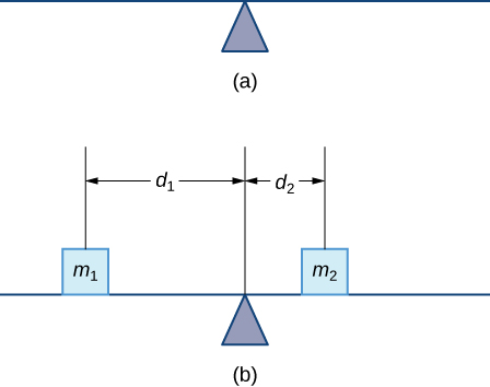
The most common real-life example of a system like this is a playground seesaw, or teeter-totter, with children of different weights sitting at different distances from the center. On a seesaw, if one child sits at each end, the heavier child sinks down and the lighter child is lifted into the air. If the heavier child slides in toward the center, though, the seesaw balances. Applying this concept to the masses on the rod, we note that the masses balance each other if and only if
\[m_1d_1=m_2d_2. \nonumber \]
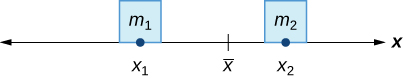
In the seesaw example, we balanced the system by moving the masses (children) with respect to the fulcrum. However, we are really interested in systems in which the masses are not allowed to move, and instead we balance the system by moving the fulcrum. Suppose we have two point masses, \(m_1\) and \(m_2\), located on a number line at points \(x_1\) and \(x_2\), respectively (Figure \(\PageIndex{2}\)). The center of mass, \(\bar{x}\), is the point where the fulcrum should be placed to make the system balance.
Thus, we have
\[ \begin{align*} m_1|x_1−\bar{x}| &=m_2|x_2−\bar{x}| \\[4pt] m_1(\bar{x}−x_1) &=m_2(x_2−\bar{x}) \\[4pt] m_1\bar{x}−m_1x_1 &=m_2x_2−m_2\bar{x} \\[4pt] \bar{x}(m_1+m_2) &=m_1x_1+m_2x_2 \end{align*} \nonumber \]
or
\[ \bar{x} =\dfrac{m_1x_1+m_2x_2}{m_1+m_2} \label{COM} \]
The expression in the numerator of Equation \ref{COM}, \(m_1x_1+m_2x_2\), is called the first moment of the system with respect to the origin. If the context is clear, we often drop the word first and just refer to this expression as the moment of the system. The expression in the denominator, \(m_1+m_2\), is the total mass of the system. Thus, the center of mass of the system is the point at which the total mass of the system could be concentrated without changing the moment.
This idea is not limited just to two point masses. In general, if \(n\) masses, \(m_1,m_2,…,m_n,\) are placed on a number line at points \(x_1,x_2,…,x_n,\) respectively, then the center of mass of the system is given by
\[ \bar{x}=\dfrac{\displaystyle {\sum_{i=1}^nm_ix_i}}{\displaystyle {\sum_{i=1}^nm_i}} \nonumber \]
Let \(m_1,m_2,…,m_n\) be point masses placed on a number line at points \(x_1,x_2,…,x_n\), respectively, and let \(\displaystyle m=\sum_{i=1}^nm_i\) denote the total mass of the system. Then, the moment of the system with respect to the origin is given by
\[M=\sum_{i=1}^nm_ix_i \label{moment} \]
and the center of mass of the system is given by
\[\bar{x}=\dfrac{M}{m}. \label{COM2a} \]
We apply this theorem in the following example.
Suppose four point masses are placed on a number line as follows:
- \(m_1=30\,kg,\) placed at \(x_1=−2m\)
- \(m_2=5\,kg,\) placed at \(x_2=3m\)
- \(m_3=10\,kg,\) placed at \(x_3=6m\)
- \(m_4=15\,kg,\) placed at \(x_4=−3m.\)
Solution
Find the moment of the system with respect to the origin and find the center of mass of the system.
First, we need to calculate the moment of the system (Equation \ref{moment}):
\[ \begin{align*} M &=\sum_{i=1}^4m_ix_i \\[4pt] &= −60+15+60−45 \\[4pt] &=−30. \end{align*}\]
Now, to find the center of mass, we need the total mass of the system:
\[ \begin{align*} m &=\sum_{i=1}^4m_i \\[4pt] &=30+5+10+15 \\[4pt] &= 60\, kg \end{align*}\]
Then we have (from Equation \ref{COM2a})
\(\bar{x}–=\dfrac{M}{m}=−\dfrac{30}{60}=−\dfrac{1}{2}\).
The center of mass is located 1/2 m to the left of the origin.
We can generalize this concept to find the center of mass of a system of point masses in a plane. Let \(m_1\) be a point mass located at point \((x_1,y_1)\) in the plane. Then the moment \(M_x\) of the mass with respect to the \(x\)-axis is given by \(M_x=m_1y_1\). Similarly, the moment \(M_y\) with respect to the \(y\)-axis is given by
\[M_y=m_1x_1. \nonumber \]
Notice that the \(x\)-coordinate of the point is used to calculate the moment with respect to the \(y\)-axis, and vice versa. The reason is that the \(x\)-coordinate gives the distance from the point mass to the \(y\)-axis, and the \(y\)-coordinate gives the distance to the \(x\)-axis (see the following figure).
If we have several point masses in the \(xy\)-plane, we can use the moments with respect to the \(x\)- and \(y\)-axes to calculate the \(x\)- and \(y\)-coordinates of the center of mass of the system.
Let \(m_1\), \(m_2\), …, \(m_n\) be point masses located in the \(xy\)-plane at points \((x_1,y_1),(x_2,y_2),…,(x_n,y_n),\) respectively, and let \(\displaystyle m=\sum_{i=1}^nm_i\) denote the total mass of the system. Then the moments \(M_x\) and \(M_y\) of the system with respect to the \(x\)- and \(y\)-axes, respectively, are given by
\[M_x=\sum_{i=1}^nm_iy_i \label{COM1} \]
and
\[M_y=\sum_{i=1}^nm_ix_i. \label{COM2} \]
Also, the coordinates of the center of mass \((\bar{x},\bar{y})\) of the system are
\[\bar{x}=\dfrac{M_y}{m} \label{COM3} \]
and
\[\bar{y}=\dfrac{M_x}{m}. \label{COM4} \]
The next example demonstrates how to the center of mass formulas (Equations \ref{COM1} - \ref{COM4}) may be applied.
Suppose three point masses are placed in the \(xy\)-plane as follows (assume coordinates are given in meters):
- \(m_1=2\,kg\) placed at \((−1,3),\)
- \(m_2=6\,kg\) placed at \((1,1),\)
- \(m_3=4\,kg\) placed at \((2,−2).\)
Find the center of mass of the system.
Solution
First we calculate the total mass of the system:
\[m=\sum_{i=1}^3m_i=2+6+4=12\,kg. \nonumber \]
Next we find the moments with respect to the \(x\)- and \(y\)-axes:
\[\begin{align*} M_y &=\sum_{i=1}^3m_ix_i=−2+6+8=12, \\[4pt] M_x &=\sum_{i=1}^3m_iy_i=6+6−8=4. \end{align*}\]
Then we have
\[\bar{x}=\dfrac{M_y}{m}=\dfrac{12}{12}=1 \nonumber \]
and
\[\bar{y}=\dfrac{M_x}{m}=\dfrac{4}{12}=\dfrac{1}{3}. \nonumber \]
The center of mass of the system is \((1,1/3),\) in meters.
Center of Mass of Thin Plates
So far we have looked at systems of point masses on a line and in a plane. Now, instead of having the mass of a system concentrated at discrete points, we want to look at systems in which the mass of the system is distributed continuously across a thin sheet of material. For our purposes, we assume the sheet is thin enough that it can be treated as if it is two-dimensional. Such a sheet is called a lamina. Next we develop techniques to find the center of mass of a lamina. In this section, we also assume the density of the lamina is constant.
Laminas are often represented by a two-dimensional region in a plane. The geometric center of such a region is called its centroid. Since we have assumed the density of the lamina is constant, the center of mass of the lamina depends only on the shape of the corresponding region in the plane; it does not depend on the density. In this case, the center of mass of the lamina corresponds to the centroid of the delineated region in the plane. As with systems of point masses, we need to find the total mass of the lamina, as well as the moments of the lamina with respect to the \(x\)- and \(y\)-axes.
We first consider a lamina in the shape of a rectangle. Recall that the center of mass of a lamina is the point where the lamina balances. For a rectangle, that point is both the horizontal and vertical center of the rectangle. Based on this understanding, it is clear that the center of mass of a rectangular lamina is the point where the diagonals intersect, which is a result of the symmetry principle, and it is stated here without proof.
If a region \(R\) is symmetric about a line \(l\), then the centroid of \(R\) lies on \(l\).
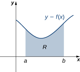
Let’s turn to more general laminas. Suppose we have a lamina bounded above by the graph of a continuous function \(f(x)\), below by the \(x\)-axis, and on the left and right by the lines \(x=a\) and \(x=b\), respectively, as shown in the following figure.
As with systems of point masses, to find the center of mass of the lamina, we need to find the total mass of the lamina, as well as the moments of the lamina with respect to the \(x\)- and \(y\)-axes. As we have done many times before, we approximate these quantities by partitioning the interval \([a,b]\) and constructing rectangles.
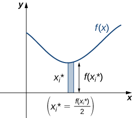
For \(i=0,1,2,…,n,\) let \(P={x_i}\) be a regular partition of \([a,b]\). Recall that we can choose any point within the interval \([x_{i−1},x_i]\) as our \(x^∗_i\). In this case, we want \(x^∗_i\) to be the x-coordinate of the centroid of our rectangles. Thus, for \(i=1,2,…,n\), we select \(x^∗_i∈[x_{i−1},x_i]\) such that \(x^∗_i\) is the midpoint of the interval. That is, \(x^∗_i=(x_{i−1}+x_i)/2\). Now, for \(i=1,2,…,n,\) construct a rectangle of height \(f(x^∗_i)\) on \([x_{i−1},x_i].\) The center of mass of this rectangle is \((x^∗_i,(f(x^∗_i))/2),\) as shown in the following figure.
Next, we need to find the total mass of the rectangle. Let \(ρ\) represent the density of the lamina (note that \(ρ\) is a constant). In this case, \(ρ\) is expressed in terms of mass per unit area. Thus, to find the total mass of the rectangle, we multiply the area of the rectangle by \(ρ\). Then, the mass of the rectangle is given by \(ρf(x^∗_i)Δx\).
To get the approximate mass of the lamina, we add the masses of all the rectangles to get
\[m≈\sum_{i=1}^nρf(x^∗_i)Δx. \label{eq51} \]
Equation \ref{eq51} is a Riemann sum. Taking the limit as \(n→∞\) gives the exact mass of the lamina:
\[ \begin{align*} m &=\lim_{n→∞}\sum_{i=1}^nρf(x^∗_i)Δx \\[4pt] &=ρ∫^b_af(x)dx. \end{align*}\]
Next, we calculate the moment of the lamina with respect to the x-axis. Returning to the representative rectangle, recall its center of mass is \((x^∗_i,(f(x^∗_i))/2)\). Recall also that treating the rectangle as if it is a point mass located at the center of mass does not change the moment. Thus, the moment of the rectangle with respect to the x-axis is given by the mass of the rectangle, \(ρf(x^∗_i)Δx\), multiplied by the distance from the center of mass to the x-axis: \((f(x^∗_i))/2\). Therefore, the moment with respect to the x-axis of the rectangle is \(ρ([f(x^∗_i)]^2/2)Δx.\) Adding the moments of the rectangles and taking the limit of the resulting Riemann sum, we see that the moment of the lamina with respect to the x-axis is
\[ \begin{align*}M_x &=\lim_{n→∞}\sum_{i=1}^nρ\dfrac{[f(x^∗_i)]^2}{2}Δx \\[4pt] &=ρ∫^b_a\dfrac{[f(x)]^2}{2}dx.\end{align*}\]
We derive the moment with respect to the y-axis similarly, noting that the distance from the center of mass of the rectangle to the y-axis is \(x^∗_i\). Then the moment of the lamina with respect to the y-axis is given by
\[ \begin{align*}M_y &=\lim_{n→∞}\sum_{i=1}^nρx^∗_if(x^∗)i)Δx\\[4pt] &=ρ∫^b_axf(x)dx.\end{align*}\]
We find the coordinates of the center of mass by dividing the moments by the total mass to give \(\bar{x}=M_y/m\) and \(\bar{y}=M_x/m\). If we look closely at the expressions for \(M_x,M_y\), and \(m\), we notice that the constant \(ρ\) cancels out when \(\bar{x}\) and \(\bar{y}\) are calculated.
We summarize these findings in the following theorem.
Let R denote a region bounded above by the graph of a continuous function \(f(x)\), below by the x-axis, and on the left and right by the lines \(x=a\) and \(x=b\), respectively. Let \(ρ\) denote the density of the associated lamina. Then we can make the following statements:
- The mass of the lamina is \[m=ρ∫^b_af(x)dx. \label{eq4a} \]
- The moments \(M_x\) and \(M_y\) of the lamina with respect to the x- and y-axes, respectively, are \[M_x=ρ∫^b_a\dfrac{[f(x)]^2}{2}dx\label{eq4b} \] and \[M_y=ρ∫^b_axf(x)dx.\label{eq4c} \]
- The coordinates of the center of mass \((\bar{x},\bar{y})\) are \[\bar{x}=\dfrac{M_y}{m} \label{eq4d} \] and \[\bar{y}=\dfrac{M_x}{m}. \label{eq4e} \]
In the next example, we use this theorem to find the center of mass of a lamina.
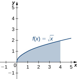
Let R be the region bounded above by the graph of the function \(f(x)=\sqrt{x}\) and below by the x-axis over the interval \([0,4]\). Find the centroid of the region.
Solution
The region is depicted in the following figure.
Since we are only asked for the centroid of the region, rather than the mass or moments of the associated lamina, we know the density constant \(ρ\) cancels out of the calculations eventually. Therefore, for the sake of convenience, let’s assume \(ρ=1\).
First, we need to calculate the total mass (Equation \ref{eq4a}):
\[ \begin{align*} m &=ρ∫^b_af(x)dx \\[4pt] &=∫^4_0\sqrt{x}dx \\[4pt] &=\dfrac{2}{3}x^{3/2}∣^4_0 \\[4pt] &=\dfrac{2}{3}[8−0] \\[4pt] &=\dfrac{16}{3}. \end{align*}\]
Next, we compute the moments (Equation \ref{eq4d}):
\[ \begin{align*} M_x &=ρ∫^b_a\dfrac{[f(x)]^2}{2}dx \\[4pt] &=∫^4_0\dfrac{x}{2}dx \\[4pt] &=\dfrac{1}{4}x^2∣^4_0 \\[4pt] &=4 \end{align*}\]
and (Equation \ref{eq4c}):
\[ \begin{align*} M_y &=ρ∫^b_axf(x)dx \\[4pt] &=∫^4_0x\sqrt{x}dx \\[4pt] &=∫^4_0x^{3/2}dx \\[4pt] &=\dfrac{2}{5}x^{5/2}∣^4_0 \\[4pt] &=\dfrac{2}{5}[32−0] \\[4pt] &=\dfrac{64}{5}. \end{align*}\]
Thus, we have (Equation \ref{eq4d}):
\[ \begin{align*} \bar{x} &=\dfrac{M_y}{m} \\[4pt] &=\dfrac{64/5}{16/3} \\[4pt] &=\dfrac{64}{5}⋅\dfrac{3}{16} \\[4pt] &=\dfrac{12}{5} \end{align*}\]
and (Equation \ref{eq4e}):
\[ \begin{align*} \bar{y} &=\dfrac{M_x}{y} \\[4pt] &=\dfrac{4}{16/3} \\[4pt] &=4⋅\dfrac{3}{16} \\[4pt] &=\dfrac{3}{4}. \end{align*}\]
The centroid of the region is \((12/5,3/4).\)
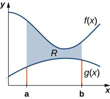
We can adapt this approach to find centroids of more complex regions as well. Suppose our region is bounded above by the graph of a continuous function \(f(x)\), as before, but now, instead of having the lower bound for the region be the x-axis, suppose the region is bounded below by the graph of a second continuous function, \(g(x)\), as shown in Figure \(\PageIndex{7}\).
Again, we partition the interval \([a,b]\) and construct rectangles. A representative rectangle is shown in Figure \(\PageIndex{8}\).
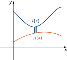
Note that the centroid of this rectangle is \((x^∗_i,(f(x^∗_i)+g(x^∗_i))/2)\). We won’t go through all the details of the Riemann sum development, but let’s look at some of the key steps. In the development of the formulas for the mass of the lamina and the moment with respect to the y-axis, the height of each rectangle is given by \(f(x^∗_i)−g(x^∗_i)\), which leads to the expression \(f(x)−g(x)\) in the integrands.
In the development of the formula for the moment with respect to the x-axis, the moment of each rectangle is found by multiplying the area of the rectangle, \(ρ[f(x^∗_i)−g(x^∗_i)]Δx,\) by the distance of the centroid from the \(x\)-axis, \((f(x^∗_i)+g(x^∗_i))/2\), which gives \(ρ(1/2){[f(x^∗_i)]^2−[g(x^∗_i)]^2}Δx\). Summarizing these findings, we arrive at the following theorem.
Let \(R\) denote a region bounded above by the graph of a continuous function \(f(x),\) below by the graph of the continuous function \(g(x)\), and on the left and right by the lines \(x=a\) and \(x=b\), respectively. Let \(ρ\) denote the density of the associated lamina. Then we can make the following statements:
- The mass of the lamina is \[m=ρ∫^b_a[f(x)−g(x)]dx. \nonumber \]
- The moments \(M_x\) and \(M_y\) of the lamina with respect to the x- and y-axes, respectively, are \[M_x=ρ∫^b_a12([f(x)]^2−[g(x)]^2)dx \nonumber \] and \[M_y=ρ∫^b_ax[f(x)−g(x)]dx. \nonumber \]
- The coordinates of the center of mass \(\bar{x},\bar{y})\) are \[\bar{x}=\dfrac{M_y}{m} \nonumber \] and \[\bar{y}=\dfrac{M_x}{m} \nonumber \]
We illustrate this theorem in the following example.
Let R be the region bounded above by the graph of the function \(f(x)=1−x^2\) and below by the graph of the function \(g(x)=x−1.\) Find the centroid of the region.
Solution
The region is depicted in the following figure.
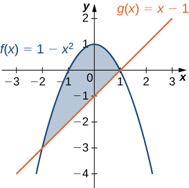
The graphs of the functions intersect at \((−2,−3)\) and \((1,0)\), so we integrate from −2 to 1. Once again, for the sake of convenience, assume \(ρ=1\).
First, we need to calculate the total mass:
\[ \begin{align*} m &=ρ∫^b_a[f(x)−g(x)]dx \\[4pt] &=∫^1_{−2}[1−x^2−(x−1)]dx \\[4pt] &=∫^1_{−2}(2−x^2−x)dx \\[4pt] &=\left[2x−\dfrac{1}{3}x^3−\dfrac{1}{2}x^2\right]∣^1_{−2} \\[4pt] &=\left[2−\dfrac{1}{3}−\dfrac{1}{2}\right]−\left[−4+\dfrac{8}{3}−2\right]\\[4pt] &=\dfrac{9}{2}. \end{align*}\]
Next, we compute the moments:
\[ \begin{align*} M_x&=ρ∫^b_a\dfrac{1}{2}([f(x)]^2−[g(x)]^2)dx \\[4pt] &=\dfrac{1}{2}∫^1_{−2}((1−x^2)^2−(x−1)^2)dx\\[4pt] &=\dfrac{1}{2}∫^1_{−2}(x^4−3x^2+2x)dx \\[4pt] &=\dfrac{1}{2} \left[\dfrac{x^5}{5}−x^3+x^2\right]∣^1_{−2}\\[4pt] &=−\dfrac{27}{10} \end{align*}\]
and
\[ \begin{align*} M_y &=ρ∫^b_ax[f(x)−g(x)]dx \\[4pt] &=∫^1_{−2}x[(1−x^2)−(x−1)]dx\\[4pt] &=∫^1_{−2}x[2−x^2−x]dx\\[4pt] &=∫^1_{−2}(2x−x^4−x^2)dx \\[4pt] &=\left[x^2−\dfrac{x^5}{5}−\dfrac{x^3}{3}\right]∣^1_{−2}\\[4pt] &=−\dfrac{9}{4}. \end{align*}\]
Therefore, we have
\[ \begin{align*} \bar{x} &=\dfrac{M_y}{m}\\[4pt] &=−\dfrac{9}{4}⋅\dfrac{2}{9}\\[4pt] &=−\dfrac{1}{2} \end{align*}\]
and
\[ \begin{align*} \bar{y} &=\dfrac{M_x}{y}\\[4pt] &=−\dfrac{27}{10}⋅\dfrac{2}{9}\\[4pt] &=−\dfrac{3}{5}. \end{align*}\]
The centroid of the region is \((−(1/2),−(3/5)).\)
The Symmetry Principle
We stated the symmetry principle earlier, when we were looking at the centroid of a rectangle. The symmetry principle can be a great help when finding centroids of regions that are symmetric. Consider the following example.
Let R be the region bounded above by the graph of the function \(f(x)=4−x^2\) and below by the x-axis. Find the centroid of the region.
Solution
The region is depicted in the following figure

The region is symmetric with respect to the y-axis. Therefore, the x-coordinate of the centroid is zero. We need only calculate \(\bar{y}\). Once again, for the sake of convenience, assume \(ρ=1\).
First, we calculate the total mass:
\[ \begin{align*} m &=ρ∫^b_af(x)dx \\[4pt] &=∫^2_{−2}(4−x^2)dx \\[4pt] &=\left[4x−\dfrac{x^3}{3}\right]∣^2_{−2} \\[4pt] &=\dfrac{32}{3}. \end{align*}\]
Next, we calculate the moments. We only need \(M_x\):
\[ \begin{align*} M_x &=ρ∫^b_a\dfrac{[f(x)]^2}{2}dx \\[4pt] &=\dfrac{1}{2}∫^2_{−2}\left[4−x^2\right]^2dx =\dfrac{1}{2}∫^2_{−2}(16−8x^2+x^4)dx \\[4pt] &=\dfrac{1}{2}\left[\dfrac{x^5}{5}−\dfrac{8x^3}{3}+16x\right]∣^2_{−2}=\dfrac{256}{15} \end{align*}\]
Then we have
\[\bar{y}=\dfrac{M_x}{y}=\dfrac{256}{15}⋅\dfrac{3}{32}=\dfrac{8}{5}. \nonumber \]
The centroid of the region is \((0,8/5).\)
The Grand Canyon Skywalk opened to the public on March 28, 2007. This engineering marvel is a horseshoe-shaped observation platform suspended 4000 ft above the Colorado River on the West Rim of the Grand Canyon. Its crystal-clear glass floor allows stunning views of the canyon below (see the following figure).
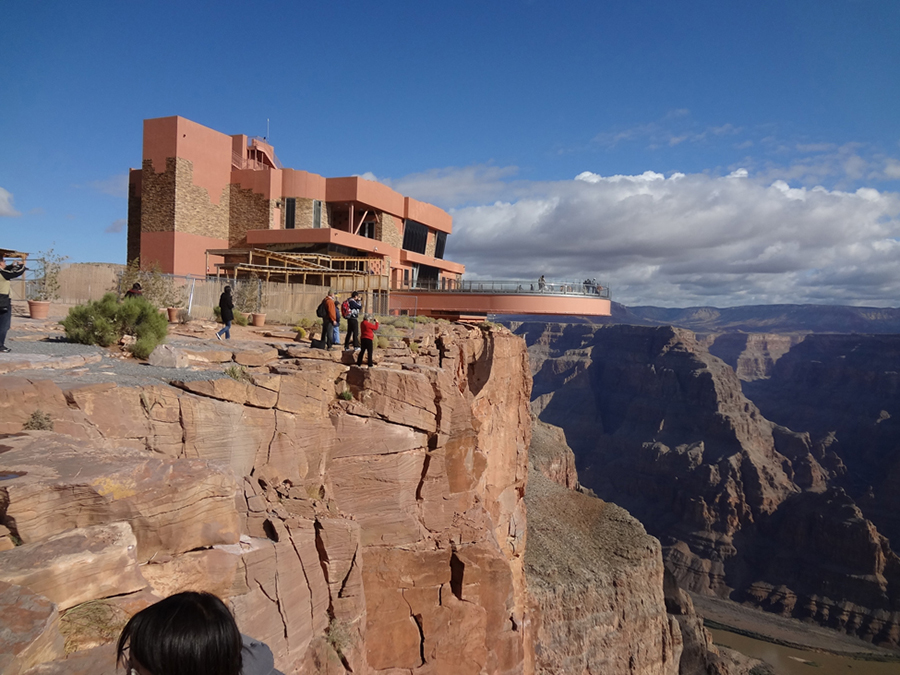
The Skywalk is a cantilever design, meaning that the observation platform extends over the rim of the canyon, with no visible means of support below it. Despite the lack of visible support posts or struts, cantilever structures are engineered to be very stable and the Skywalk is no exception. The observation platform is attached firmly to support posts that extend 46 ft down into bedrock. The structure was built to withstand 100-mph winds and an 8.0-magnitude earthquake within 50 mi, and is capable of supporting more than 70,000,000 lb.
One factor affecting the stability of the Skywalk is the center of gravity of the structure. We are going to calculate the center of gravity of the Skywalk, and examine how the center of gravity changes when tourists walk out onto the observation platform.
The observation platform is U-shaped. The legs of the U are 10 ft wide and begin on land, under the visitors’ center, 48 ft from the edge of the canyon. The platform extends 70 ft over the edge of the canyon.
To calculate the center of mass of the structure, we treat it as a lamina and use a two-dimensional region in the xy-plane to represent the platform. We begin by dividing the region into three subregions so we can consider each subregion separately. The first region, denoted \(R_1\), consists of the curved part of the U. We model \(R_1\) as a semicircular annulus, with inner radius 25 ft and outer radius 35 ft, centered at the origin (Figure \(\PageIndex{12}\)).
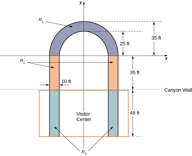
The legs of the platform, extending 35 ft between \(R_1\) and the canyon wall, comprise the second sub-region, \(R_2\). Last, the ends of the legs, which extend 48 ft under the visitor center, comprise the third sub-region, \(R_3\). Assume the density of the lamina is constant and assume the total weight of the platform is 1,200,000 lb (not including the weight of the visitor center; we will consider that later). Use \(g=32\;ft/sec^2\).
- Compute the area of each of the three sub-regions. Note that the areas of regions \(R_2\) and \(R_3\) should include the areas of the legs only, not the open space between them. Round answers to the nearest square foot.
- Determine the mass associated with each of the three sub-regions.
- Calculate the center of mass of each of the three sub-regions.
- Now, treat each of the three sub-regions as a point mass located at the center of mass of the corresponding sub-region. Using this representation, calculate the center of mass of the entire platform.
- Assume the visitor center weighs 2,200,000 lb, with a center of mass corresponding to the center of mass of \(R_3\).Treating the visitor center as a point mass, recalculate the center of mass of the system. How does the center of mass change?
- Although the Skywalk was built to limit the number of people on the observation platform to 120, the platform is capable of supporting up to 800 people weighing 200 lb each. If all 800 people were allowed on the platform, and all of them went to the farthest end of the platform, how would the center of gravity of the system be affected? (Include the visitor center in the calculations and represent the people by a point mass located at the farthest edge of the platform, 70 ft from the canyon wall.)
Theorem of Pappus
This section ends with a discussion of the theorem of Pappus for volume, which allows us to find the volume of particular kinds of solids by using the centroid. (There is also a theorem of Pappus for surface area, but it is much less useful than the theorem for volume.)
Let \(R\) be a region in the plane and let l be a line in the plane that does not intersect \(R\). Then the volume of the solid of revolution formed by revolving \(R\) around l is equal to the area of \(R\) multiplied by the distance d traveled by the centroid of \(R\).
We can prove the case when the region is bounded above by the graph of a function \(f(x)\) and below by the graph of a function \(g(x)\) over an interval \([a,b]\), and for which the axis of revolution is the \(y\)-axis. In this case, the area of the region is \(\displaystyle A=∫^b_a[f(x)−g(x)]\,dx\). Since the axis of rotation is the \(y\)-axis, the distance traveled by the centroid of the region depends only on the \(x\)-coordinate of the centroid, \(\bar{x}\), which is
\[x=\dfrac{M_y}{m}, \nonumber \]
where
\[m=ρ∫^b_a[f(x)−g(x)]dx \nonumber \]
and
\[M_y=ρ∫^b_ax[f(x)−g(x)]dx. \nonumber \]
Then,
\[d=2π\dfrac{\displaystyle {ρ∫^b_ax[f(x)−g(x)]dx}}{\displaystyle{ρ∫^b_a[f(x)−g(x)]dx}} \nonumber \]
and thus
\[d⋅A=2π∫^b_ax[f(x)−g(x)]dx. \nonumber \]
However, using the method of cylindrical shells, we have
\[V=2π∫^b_ax[f(x)−g(x)]dx. \nonumber \]
So,
\[V=d⋅A \nonumber \]
and the proof is complete.
□
Let \(R\) be a circle of radius 2 centered at \((4,0).\) Use the theorem of Pappus for volume to find the volume of the torus generated by revolving \(R\) around the \(y\)-axis.
Solution
The region and torus are depicted in the following figure.
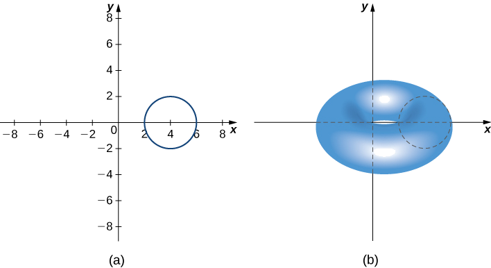
The region \(R\) is a circle of radius 2, so the area of R is \(A=4π\;\text{units}^2\). By the symmetry principle, the centroid of R is the center of the circle. The centroid travels around the \(y\)-axis in a circular path of radius 4, so the centroid travels \(d=8π\) units. Then, the volume of the torus is \(A⋅d=32π^2\) units3.
We have already discussed a few applications of multiple integrals, such as finding areas, volumes, and the average value of a function over a bounded region. In this section we develop computational techniques for finding the center of mass and moments of inertia of several types of physical objects, using double integrals for a lamina (flat plate) and triple integrals for a three-dimensional object with variable density. The density is usually considered to be a constant number when the lamina or the object is homogeneous; that is, the object has uniform density.
Center of Mass in Two Dimensions
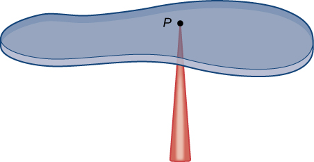
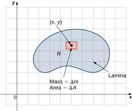
The center of mass is also known as the center of gravity if the object is in a uniform gravitational field. If the object has uniform density, the center of mass is the geometric center of the object, which is called the centroid. Figure \(\PageIndex{1}\) shows a point \(P\) as the center of mass of a lamina. The lamina is perfectly balanced about its center of mass.
To find the coordinates of the center of mass \(P(\bar{x},\bar{y})\) of a lamina, we need to find the moment \(M_x\) of the lamina about the \(x\)-axis and the moment \(M_y\) about the \(y\)-axis. We also need to find the mass \(m\) of the lamina. Then
\[\bar{x} = \dfrac{M_y}{m} \nonumber \]
and
\[\bar{y} = \dfrac{M_x}{m}. \nonumber \]
Refer to Moments and Centers of Mass for the definitions and the methods of single integration to find the center of mass of a one-dimensional object (for example, a thin rod). We are going to use a similar idea here except that the object is a two-dimensional lamina and we use a double integral.
If we allow a constant density function, then \(\bar{x} = \dfrac{M_y}{m}\) and \(\bar{y} = \dfrac{M_x}{m}\) give the centroid of the lamina.
Suppose that the lamina occupies a region \(R\) in the \(xy\)-plane and let \(\rho (x,y)\) be its density (in units of mass per unit area) at any point \((x,y)\). Hence,
\[\rho(x,y) = \lim_{\Delta A \rightarrow 0} \dfrac{\Delta m}{\Delta A} \nonumber \]
where \(\Delta m\) and \(\Delta A\) are the mass and area of a small rectangle containing the point \((x,y)\) and the limit is taken as the dimensions of the rectangle go to \(0\) (see the following figure).
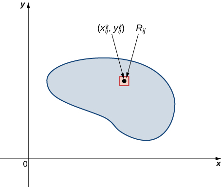
Just as before, we divide the region \(R\) into tiny rectangles \(R_{ij}\) with area \(\Delta A\) and choose \((x_{ij}^*, y_{ij}^*)\) as sample points. Then the mass \(m_{ij}\) of each \(R_{ij}\) is equal to \(\rho (x_{ij}^*, y_{ij}^*) \Delta A\) (Figure \(\PageIndex{2}\)). Let \(k\) and \(l\) be the number of subintervals in \(x\) and \(y\) respectively. Also, note that the shape might not always be rectangular but the limit works anyway, as seen in previous sections.
Hence, the mass of the lamina is
\[m =\lim_{k,l \rightarrow \infty} \sum_{i=1}^k \sum_{j=1}^l m_{ij} = \lim_{k,l \rightarrow \infty} \sum_{i=1}^k \sum_{j=1}^l \rho(x_{ij}^*,y_{ij}^*) \Delta A = \iint_R \rho(x,y) dA. \nonumber \]
Let’s see an example now of finding the total mass of a triangular lamina.
Consider a triangular lamina \(R\) with vertices \((0,0), \, (0,3), \, (3,0)\) and with density \(\rho(x,y) = xy \, kg/m^2\). Find the total mass.
- Solution:
-
A sketch of the region \(R\) is always helpful, as shown in the following figure.
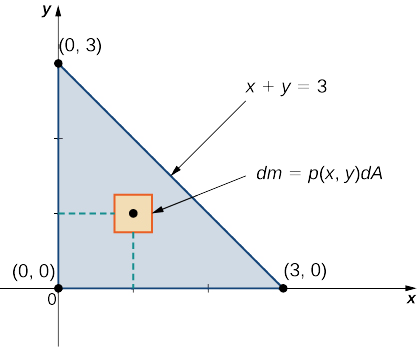
Figure \(\PageIndex{4}\): A lamina in the \(xy\)-plane with density \(\rho (x,y) = xy\). Using the expression developed for mass, we see that
\[m = \iint_R \, dm = \iint_R \rho (x,y) dA = \int_{x=0}^{x=3} \int_{y=0}^{y=3-x} xy \, dy \, dx = \int_{x=0}^{x=3} \left[ \left. x \dfrac{y^2}{2} \right|_{y=0}^{y=3} \right] \, dx = \int_{x=0}^{x=3} \dfrac{1}{2} x (3 - x)^2 dx = \left.\left[ \dfrac{9x^2}{4} - x^3 + \dfrac{x^4}{8} \right]\right|_{x=0}^{x=3} = \dfrac{27}{8}. \nonumber \]
The computation is straightforward, giving the answer \(m = \dfrac{27}{8} \, kg\).
Now that we have established the expression for mass, we have the tools we need for calculating moments and centers of mass. The moment \(M_z\) about the \(x\)-axis for \(R\) is the limit of the sums of moments of the regions \(R_{ij}\) about the \(x\)-axis. Hence
\[M_x = \lim_{k,l \rightarrow \infty} \sum_{i=1}^k \sum_{j=1}^l (y_{ij}^*)m_{ij} = \lim_{k,l \rightarrow \infty} \sum_{i=1}^k \sum_{j=1}^l (y_{ij}^*) \rho(x_{ij}^*,y_{ij}^*) \,\Delta A = \iint_R y\rho (x,y) \,dA \nonumber \]
Similarly, the moment \(M_y\) about the \(y\)-axis for \(R\) is the limit of the sums of moments of the regions \(R_{ij}\) about the \(y\)-axis. Hence
\[M_y = \lim_{k,l \rightarrow \infty} \sum_{i=1}^k \sum_{j=1}^l (x_{ij}^*)m_{ij} = \lim_{k,l \rightarrow \infty} \sum_{i=1}^k \sum_{j=1}^l (x_{ij}^*) \rho(x_{ij}^*,y_{ij}^*) \,\Delta A = \iint_R x\rho (x,y) \,dA \nonumber \]
Consider the same triangular lamina \(R\) with vertices \((0,0), \, (0,3), \, (3,0)\) and with density \(\rho (x,y) = xy\). Find the moments \(M_x\) and \(M_y\).
- Solution:
-
Use double integrals for each moment and compute their values:
\[M_x = \iint_R y\rho (x,y) \,dA = \int_{x=0}^{x=3} \int_{y=0}^{y=3-x} x y^2 \, dy \, dx = \dfrac{81}{20}, \nonumber \]
\[M_y = \iint_R x\rho (x,y) \,dA = \int_{x=0}^{x=3} \int_{y=0}^{y=3-x} x^2 y \, dy \, dx = \dfrac{81}{20}, \nonumber \]
The computation is quite straightforward.
Finally we are ready to restate the expressions for the center of mass in terms of integrals. We denote the x-coordinate of the center of mass by \(\bar{x}\) and the y-coordinate by \(\bar{y}\). Specifically,
\[\bar{x} = \dfrac{M_y}{m} = \dfrac{\iint_R x\rho (x,y) \,dA}{\iint_R \rho (x,y)\,dA} \nonumber \]
and
\[\bar{y} = \dfrac{M_x}{m} = \dfrac{\iint_R y\rho (x,y) \,dA}{\iint_R \rho (x,y)\,dA} \nonumber \]
Again consider the same triangular region \(R\) with vertices \((0,0), \, (0,3), \, (3,0)\) and with density function \(\rho (x,y) = xy\). Find the center of mass.
- Solution:
-
Using the formulas we developed, we have
\[\bar{x} = \dfrac{M_y}{m} = \dfrac{\iint_R x\rho (x,y) \,dA}{\iint_R \rho (x,y)\,dA} = \dfrac{81/20}{27/8} = \dfrac{6}{5}, \nonumber \]
\[\bar{y} = \dfrac{M_x}{m} = \dfrac{\iint_R y\rho (x,y) \,dA}{\iint_R \rho (x,y)\,dA} = \dfrac{81/20}{27/8} = \dfrac{6}{5}. \nonumber \]
Therefore, the center of mass is the point \(\left(\dfrac{6}{5},\dfrac{6}{5}\right).\)
Analysis
If we choose the density \(\rho(x,y)\) instead to be uniform throughout the region (i.e., constant), such as the value 1 (any constant will do), then we can compute the centroid,
\[x_c = \dfrac{M_y}{m} = \dfrac{\iint_R x \, dA}{\iint_R \,dA} = \dfrac{9/2}{9/2} = 1, \nonumber \]
\[y_c = \dfrac{M_x}{m} = \dfrac{\iint_R y \, dA}{\iint_R \,dA} = \dfrac{9/2}{9/2} = 1. \nonumber \]
Notice that the center of mass \(\left(\dfrac{6}{5},\dfrac{6}{5}\right)\) is not exactly the same as the centroid \((1,1)\) of the triangular region. This is due to the variable density of \(R\) If the density is constant, then we just use \(\rho(x,y) = c\) (constant). This value cancels out from the formulas, so for a constant density, the center of mass coincides with the centroid of the lamina.
Once again, based on the comments at the end of Example \(\PageIndex{3}\), we have expressions for the centroid of a region on the plane:
\[x_c = \dfrac{M_y}{m} = \dfrac{\iint_R x \, dA}{\iint_R \,dA} \, \text{and} \, y_c = \dfrac{M_x}{m} = \dfrac{\iint_R y \, dA}{\iint_R \,dA}. \nonumber \]
We should use these formulas and verify the centroid of the triangular region R referred to in the last three examples.
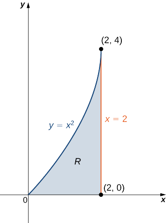
Find the mass, moments, and the center of mass of the lamina of density \(\rho(x,y) = x + y\) occupying the region \(R\) under the curve \(y = x^2\) in the interval \(0 \leq x \leq 2\) (see the following figure).
- Solution:
-
First we compute the mass \(m\). We need to describe the region between the graph of \(y = x^2\) and the vertical lines \(x = 0\) and \(x = 2\):
\[m = \iint_R \,dm = \iint_R \rho (x,y) \,dA = \int_{x=0}{x=2} \int_{y=0}^{y=x^2} (x + y) dy \, dx = \int_{x=0}^{x=2} \left[\left. xy + \dfrac{y^2}{2}\right|_{y=0}^{y=x^2} \right] \,dx \nonumber \]
\[= \int_{x=0}^{x=2} \left[ x^3 + \dfrac{x^4}{2} \right] dx = \left.\left[ \dfrac{x^4}{4} + \dfrac{x^5}{10}\right] \right|_{x=0}^{x=2} = \dfrac{36}{5}. \nonumber \]
Now compute the moments \(M_x\) and \(M_y\):
\[M_x = \iint_R y \rho (x,y) \,dA = \int_{x=0}^{x=2} \int_{y=0}^{y=x^2} y(x + y) \,dy \, dx = \dfrac{80}{7}, \nonumber \]
\[M_y = \iint_R x \rho (x,y) \,dA = \int_{x=0}^{x=2} \int_{y=0}^{y=x^2} x(x + y) \,dy \, dx = \dfrac{176}{15}. \nonumber \]
Finally, evaluate the center of mass,
\[\bar{x} = \dfrac{M_y}{m} = \dfrac{\iint_R x \rho (x,y) \,dA}{\iint_R \rho (x,y)\,dA} = \dfrac{176/15}{36/5} = \dfrac{44}{27}, \nonumber \]
\[\bar{y} = \dfrac{M_x}{m} = \dfrac{\iint_R y \rho (x,y) \,dA}{\iint_R \rho (x,y)\,dA} = \dfrac{80/7}{36/5} = \dfrac{100}{63}. \nonumber \]
Hence the center of mass is \((\bar{x},\bar{y}) = \left(\dfrac{44}{27}, \dfrac{100}{63} \right)\).
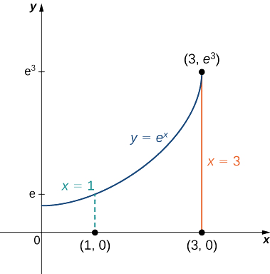
Find the centroid of the region under the curve \(y = e^x\) over the interval \(1 \leq x \leq 3\) (Figure \(\PageIndex{6}\)).
- Solution:
-
To compute the centroid, we assume that the density function is constant and hence it cancels out:
\[x_c = \dfrac{M_y}{m} = \dfrac{\iint_R x \, dA}{\iint_R dA} \, and \, y_c = \dfrac{M_x}{m} = \dfrac{\iint_R y \, dA}{\iint_R dA}, \nonumber \]
\[x_c = \dfrac{M_y}{m} = \dfrac{\iint_R x \, dA}{\iint_R dA} = \dfrac{\int_{x=1}^{x=3} \int_{y=0}^{y=e^x} x \, dy \, dx}{\int_{x=1}^{x=3} \int_{y=0}^{y=e^x} \,dy \, dx} = \dfrac{\int_{x=1}^{x=3} xe^x dx}{\int_{x=1}^{x=3} e^x dx} = \dfrac{2e^3}{e^3 - e} = \dfrac{2e^2}{e^2 - 1}, \nonumber \]
\[y_c = \dfrac{M_x}{m} = \dfrac{\iint_R y \, dA}{\iint_R dA} = \dfrac{\int_{x=1}^{x=3} \int_{y=0}^{y=e^x} y \, dy \, dx}{\int_{x=1}^{x=3} \int_{y=0}^{y=e^x} \,dy \, dx} = \dfrac{\int_{x=1}^{x=3} \dfrac{e^{2x}}{2} dx}{\int_{x=1}^{x=3} e^x dx} =\dfrac{\dfrac{1}{4} e^2 (e^4 - 1)}{e(e^2 - 1)} = \dfrac{1}{4} e(e^2 + 1). \nonumber \]
Thus the centroid of the region is
\[(x_c,y_c) = \left( \dfrac{2e^2}{e^2 - 1}, \dfrac{1}{4} e(e^2 + 1)\right). \nonumber \]
Moment of Inertia
We defined the moment of inertia I of an object to be
\[I = \sum_{i} m_i r_i^2 \]
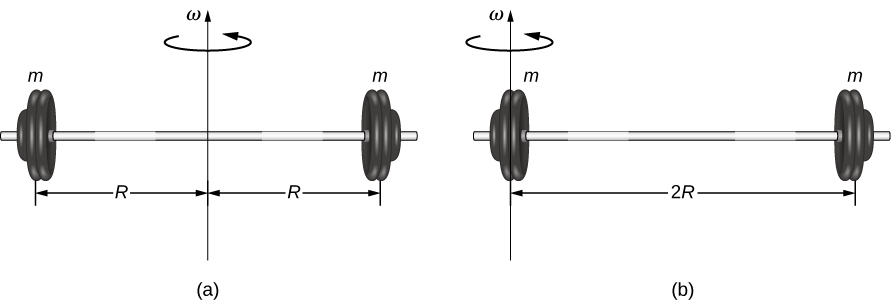
for all the point masses that make up the object. Because \(r\) is the distance to the axis of rotation from each piece of mass that makes up the object, the moment of inertia for any object depends on the chosen axis. To see this, let’s take a simple example of two masses at the end of a massless (negligibly small mass) rod (Figure \(\PageIndex{1}\)) and calculate the moment of inertia about two different axes. In this case, the summation over the masses is simple because the two masses at the end of the barbell can be approximated as point masses, and the sum therefore has only two terms.
In the case with the axis in the center of the barbell, each of the two masses m is a distance \(R\) away from the axis, giving a moment of inertia of
\[I_{1} = mR^{2} + mR^{2} = 2mR^{2} \ldotp\]
In the case with the axis at the end of the barbell—passing through one of the masses—the moment of inertia is
\[I_{2} = m(0)^{2} + m(2R)^{2} = 4mR^{2} \ldotp\]
From this result, we can conclude that it is twice as hard to rotate the barbell about the end than about its center.
In this example, we had two point masses and the sum was simple to calculate. However, to deal with objects that are not point-like, we need to think carefully about each of the terms in the equation. The equation asks us to sum over each ‘piece of mass’ a certain distance from the axis of rotation. But what exactly does each ‘piece of mass’ mean? Recall that in our derivation of this equation, each piece of mass had the same magnitude of velocity, which means the whole piece had to have a single distance r to the axis of rotation. However, this is not possible unless we take an infinitesimally small piece of mass dm, as shown in Figure \(\PageIndex{2}\).
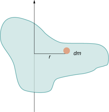
The need to use an infinitesimally small piece of mass dm suggests that we can write the moment of inertia by evaluating an integral over infinitesimal masses rather than doing a discrete sum over finite masses:
\[I = \sum_{i} m_{i} r_{i}^{2}\]
becomes
\[I = \int r^{2} dm \ldotp \label{10.19}\]
This, in fact, is the form we need to generalize the equation for complex shapes. It is best to work out specific examples in detail to get a feel for how to calculate the moment of inertia for specific shapes. This is the focus of most of the rest of this section.
A uniform thin rod with an axis through the center
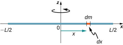
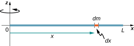
Consider a uniform (density and shape) thin rod of mass M and length L as shown in Figure \(\PageIndex{3}\). We want a thin rod so that we can assume the cross-sectional area of the rod is small and the rod can be thought of as a string of masses along a one-dimensional straight line. In this example, the axis of rotation is perpendicular to the rod and passes through the midpoint for simplicity. Our task is to calculate the moment of inertia about this axis. We orient the axes so that the z-axis is the axis of rotation and the x-axis passes through the length of the rod, as shown in the figure. This is a convenient choice because we can then integrate along the x-axis.
We define dm to be a small element of mass making up the rod. The moment of inertia integral is an integral over the mass distribution. However, we know how to integrate over space, not over mass. We therefore need to find a way to relate mass to spatial variables. We do this using the linear mass density \(\lambda\) of the object, which is the mass per unit length. Since the mass density of this object is uniform, we can write
\[\lambda = \frac{m}{l}\; or\; m = \lambda l \ldotp\]
If we take the differential of each side of this equation, we find
\[dm = d(\lambda l) = \lambda (dl)\]
since \(\lambda\) is constant. We chose to orient the rod along the x-axis for convenience—this is where that choice becomes very helpful. Note that a piece of the rod dl lies completely along the x-axis and has a length dx; in fact, dl = dx in this situation. We can therefore write dm = \(\lambda\)(dx), giving us an integration variable that we know how to deal with. The distance of each piece of mass dm from the axis is given by the variable x, as shown in the figure. Putting this all together, we obtain
\[I = \int r^{2} dm = \int x^{2} dm = \int x^{2} \lambda dx \ldotp\]
The last step is to be careful about our limits of integration. The rod extends from x = \(− \frac{L}{2}\) to x = \(\frac{L}{2}\), since the axis is in the middle of the rod at x = 0. This gives us
\[\begin{split} I & = \int_{- \frac{L}{2}}^{\frac{L}{2}} x^{2} \lambda dx = \lambda \frac{x^{3}}{3} \Bigg|_{- \frac{L}{2}}^{\frac{L}{2}} \\ & = \lambda \left(\dfrac{1}{3}\right) \Bigg[ \left(\dfrac{L}{2}\right)^{3} - \left(- \dfrac{L}{2}\right)^{3} \Bigg] = \lambda \left(\dfrac{1}{3}\right) \left(\dfrac{L^{3}}{8}\right) (2) = \left(\dfrac{M}{L}\right) \left(\dfrac{1}{3}\right) \left(\dfrac{L^{3}}{8}\right) (2) \\ & = \frac{1}{12} ML^{2} \ldotp \end{split}\]
Next, we calculate the moment of inertia for the same uniform thin rod but with a different axis choice so we can compare the results. We would expect the moment of inertia to be smaller about an axis through the center of mass than the endpoint axis, just as it was for the barbell example at the start of this section. This happens because more mass is distributed farther from the axis of rotation.
A Uniform Thin Rod with Axis at the End
Now consider the same uniform thin rod of mass \(M\) and length \(L\), but this time we move the axis of rotation to the end of the rod. We wish to find the moment of inertia about this new axis (Figure \(\PageIndex{4}\)).
The quantity \(dm\) is again defined to be a small element of mass making up the rod. Just as before, we obtain
\[I = \int r^{2} dm = \int x^{2} dm = \int x^{2} \lambda dx \ldotp\]
However, this time we have different limits of integration. The rod extends from \(x = 0\) to \(x = L\), since the axis is at the end of the rod at \(x = 0\). Therefore we find
\[\begin{align} I & = \int_{0}^{L} x^{2} \lambda\, dx \\[4pt] &= \lambda \frac{x^{3}}{3} \Bigg|_{0}^{L} \\[4pt] &=\lambda \left(\dfrac{1}{3}\right) \Big[(L)^{3} - (0)^{3} \Big] \\[4pt] & = \lambda \left(\dfrac{1}{3}\right) L^{3} = \left(\dfrac{M}{L}\right) \left(\dfrac{1}{3}\right) L^{3} \\[4pt] &= \frac{1}{3} ML^{2} \ldotp \label{ThinRod} \end{align} \]
Note the rotational inertia of the rod about its endpoint is larger than the rotational inertia about its center (consistent with the barbell example) by a factor of four.
A Uniform Thin Disk about an Axis through the Center
Integrating to find the moment of inertia of a two-dimensional object is a little bit trickier, but one shape is commonly done at this level of study—a uniform thin disk about an axis through its center (Figure \(\PageIndex{5}\)).
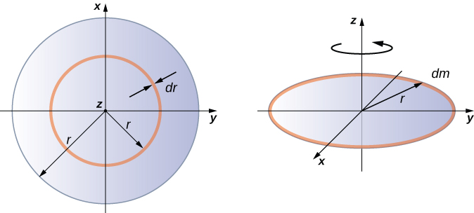
Since the disk is thin, we can take the mass as distributed entirely in the xy-plane. We again start with the relationship for the surface mass density, which is the mass per unit surface area. Since it is uniform, the surface mass density \(\sigma\) is constant:
\[\sigma = \frac{m}{A}\] or \[\sigma A = m\] so \[dm = \sigma (dA)\]
Now we use a simplification for the area. The area can be thought of as made up of a series of thin rings, where each ring is a mass increment dm of radius \(r\) equidistant from the axis, as shown in part (b) of the figure. The infinitesimal area of each ring \(dA\) is therefore given by the length of each ring (\(2 \pi r\)) times the infinitesimmal width of each ring \(dr\):
\[A = \pi r^{2},\; dA = d(\pi r^{2}) = \pi dr^{2} = 2 \pi rdr \ldotp\]
The full area of the disk is then made up from adding all the thin rings with a radius range from \(0\) to \(R\). This radius range then becomes our limits of integration for \(dr\), that is, we integrate from \(r = 0\) to \(r = R\). Putting this all together, we have
\[\begin{split} I & = \int_{0}^{R} r^{2} \sigma (2 \pi r) dr = 2 \pi \sigma \int_{0}^{R} r^{3} dr = 2 \pi \sigma \frac{r^{4}}{4} \Big|_{0}^{R} \\ & = 2 \pi \sigma \left(\dfrac{R^{4}}{4} - 0 \right) = 2 \pi \left(\dfrac{m}{A}\right) \left(\dfrac{R^{4}}{4}\right) = 2 \pi \left(\dfrac{m}{\pi R^{2}}\right) \left(\dfrac{R^{4}}{4}\right) = \frac{1}{2} mR^{2} \ldotp \end{split}\]
Note that this agrees with the value given in Figure 10.5.4.
I shall now derive the first three of these by calculus. The derivations for the spheres will be left until later.
1.Rod, length \( 2l \) (Figure II.2)
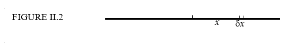
The mass of an element \(\delta x\) at a distance \( x \) from the middle of the rod is \( \dfrac{m\delta x}{2l}\).
and its second moment of inertia is
\[ \dfrac{mx^{2}\delta x}{2l}. \nonumber \]
\[\dfrac{m}{2l} \int_{-l}^{l} x^{2} dx = \dfrac{m}{l} \int_0^l x^{2} dx = \dfrac{1}{3}ml^{2}. \nonumber \]
2. Disc, radius \( a\) . (Figure II.3)
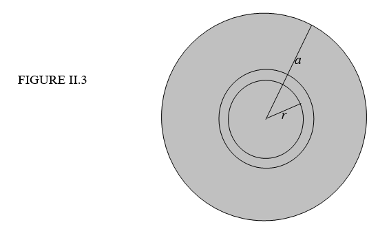
The area of an elemental annulus, radii \( r \) is \(r + \delta r \) is \(2 \pi r \delta r\).
The area of the entire disc is \(\pi a^{2} \).
Therefore the mass of the annulus is
\[\dfrac{2 \pi r \delta rm}{\pi a^{2}} = \dfrac{2mr\delta r}{a^{2} } . \nonumber \]
and its second moment of inertia is
\[\dfrac{2mr^{3}\delta r}{a^{2}}. \nonumber \]
The moment of inertia of the entire disc is
\[\dfrac{2m}{a^{2}} \int_{0}^{a} r^{3} dr = \dfrac{1}{2}ma^{2}. \nonumber \]
3. Right-angled triangular lamina. (Figure II.4)
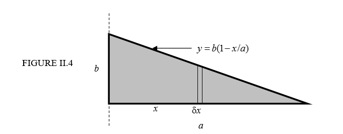
The equation to the hypotenuse is \(y = b(1 - x/a)\).
The area of the elemental strip is \(y \delta x = b(1 - x/a)\delta x \) and the area of the entire triangle is \( \dfrac{ab}{2} \).
Therefore the mass of the elemental strip is \( \dfrac{2m(a - x)\delta x}{a^{2}}\).
and its second moment of inertia is \( \dfrac{2mx^{2}(a - x)\delta x}{a^{2}}\).
The second moment of inertia of the entire triangle is the integral of this from \( x = 0 \) to \( x = a\) , which is \( \dfrac{ma^{2}}{6} \).
Uniform circular lamina about a diameter.
For the sake of one more bit of integration practice, we shall now use the same argument to show that the moment of inertia of a uniform circular disc about a diameter is \( \dfrac{ma^{2}}{4}\). However, we shall see later that it is not necessary to resort to integral calculus to arrive at this result, nor is it necessary to commit the result to memory. In a little while it will become immediately apparent and patently obvious, with no calculation, that the moment of inertia must be \( \dfrac{ma^{2}}{4}\). However, for the time being, let us have some more calculus practice. See Figure II.5.
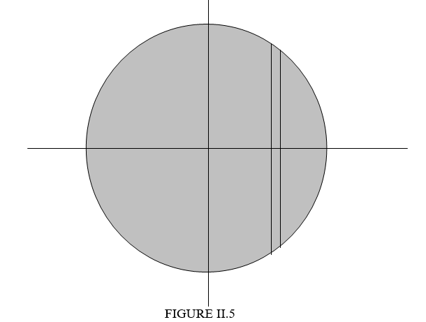
The disc is of radius \( a \), and the area of the elemental strip is \( 2y \delta x\). But \( y \) and \( x \) are related through the equation to the circle, which is \( y=(a^{2}-x^{2})^{1/2}\). Therefore the area of the strip is \( 2(a^{2} - x^{x})^{1/2} \delta x \). The area of the whole disc is \(\pi a^{2}\), so the mass of the strip is
\[m \times \dfrac{2(a^{2} - x^{2})^{1/2}\delta x}{\pi a^{2}} = \dfrac{2m}{\pi a^{2}} \times (a^{2} - x^{2})^{1/2}\delta x. \nonumber \]
The second moment of inertia about the \(y\)-axis is
\[\dfrac{2m}{\pi a^{2}} \times x^{2}(a^{2} - x^{2})^{1/2}\delta x. \nonumber \]
For the entire disc, we integrate from \( x = -a \) to \( x = +a \), or, if you prefer, from \( x = 0 \) to \( x = a \) and then double it. The result \( \dfrac{ma^{2}}{4} \) should follow. If you need a hint about how to do the integration, let \( x = a cos \theta \) (which it is, anyway), and be sure to get the limits of integration with respect to \(\theta\) right.
The moment of inertia of a uniform semicircular lamina of mass \( m \) and radius \( a \) about its base, or diameter, is also \( \dfrac{ma^{2}}{4} \), since the mass distribution with respect to rotation about the diameter is the same. \( \dfrac{ma^{2}}{4} \), since the mass distribution with respect to rotation about the diameter is the same.
Moments of Inertia
For a clear understanding of how to calculate moments of inertia using double integrals, we need to go back to the general definition in Section \(6.6\). The moment of inertia of a particle of mass \(m\) about an axis is \(mr^2\) where \(r\) is the distance of the particle from the axis. We can see from Figure \(\PageIndex{3}\) that the moment of inertia of the subrectangle \(R_{ij}\) about the \(x\)-axis is \((y_{ij}^*)^2 \rho(x_{ij}^*,y_{ij}^*) \Delta A\). Similarly, the moment of inertia of the subrectangle \(R_{ij}\) about the \(y\)-axis is \((x_{ij}^*)^2 \rho(x_{ij}^*,y_{ij}^*) \Delta A\). The moment of inertia is related to the rotation of the mass; specifically, it measures the tendency of the mass to resist a change in rotational motion about an axis.
The moment of inertia \(I_x\) about the \(x\)-axis for the region \(R\) is the limit of the sum of moments of inertia of the regions \(R_{ij}\) about the \(x\)-axis. Hence
\[I_x = \lim_{k,l\rightarrow \infty} \sum_{i=1}^k \sum_{j=1}^l (y_{ij}^*)^2 m_{ij} = \lim_{k,l\rightarrow \infty} \sum_{i=1}^k \sum_{j=1}^l (y_{ij}^*)^2 \rho (x_{ij}^*, y_{ij}^*) \,\Delta A = \iint_R y^2 \rho(x,y)\,dA. \nonumber \]
Similarly, the moment of inertia \(I_y\) about the \(y\)-axis for \(R\) is the limit of the sum of moments of inertia of the regions \(R_{ij}\) about the \(y\)-axis. Hence
\[I_y = \lim_{k,l\rightarrow \infty} \sum_{i=1}^k \sum_{j=1}^l (x_{ij}^*)^2 m_{ij} = \lim_{k,l\rightarrow \infty} \sum_{i=1}^k \sum_{j=1}^l (x_{ij}^*)^2 \rho (x_{ij}^*, y_{ij}^*) \,\Delta A = \iint_R x^2 \rho(x,y)\,dA. \nonumber \]
Sometimes, we need to find the moment of inertia of an object about the origin, which is known as the polar moment of inertia. We denote this by \(I_0\) and obtain it by adding the moments of inertia \(I_x\) and \(I_y\). Hence
\[I_0 = I_x + I_y = \iint_R (x^2 + y^2) \rho (x,y) \,dA. \nonumber \]
All these expressions can be written in polar coordinates by substituting \(x = r \, \cos \, \theta, \, y = r \, \sin \, \theta\), and \(dA = r \, dr \, d\theta\). For example, \(I_0 = \iint_R r^2 \rho (r \, \cos \, \theta, \, r \, \sin \, \theta)\,dA\).
Use the triangular region \(R\) with vertices \((0,0), \, (2,2)\), and \((2,0)\) and with density \(\rho (x,y) = xy\) as in previous examples. Find the moments of inertia.
- Solution:
-
Using the expressions established above for the moments of inertia, we have
\[I_x = \iint_R y^2 \rho(x,y) \,dA = \int_{x=0}^{x=2} \int_{y=0}^{y=x} xy^3 \,dy \, dx = \dfrac{8}{3}, \nonumber \]
\[I_y = \iint_R x^2 \rho(x,y) \,dA = \int_{x=0}^{x=2} \int_{y=0}^{y=x} x^3y \,dy \, dx = \dfrac{16}{3}, \nonumber \]
\[I_0 = \iint_R (x^2 + y^2) \rho(x,y) \,dA = \int_0^2 \int_0^x (x^2 + y^2) xy \, dy \, dx = I_x + I_y = 8 \nonumber \]
As mentioned earlier, the moment of inertia of a particle of mass \(m\) about an axis is \(mr^2\) where \(r\) is the distance of the particle from the axis, also known as the radius of gyration.
Hence the radii of gyration with respect to the \(x\)-axis, the \(y\)-axis and the origin are
\[R_x = \sqrt{\dfrac{I_x}{m}}, \, R_y = \sqrt{\dfrac{I_y}{m}}, \, and \, R_0 = \sqrt{\dfrac{I_0}{m}}, \nonumber \]
respectively. In each case, the radius of gyration tells us how far (perpendicular distance) from the axis of rotation the entire mass of an object might be concentrated. The moments of an object are useful for finding information on the balance and torque of the object about an axis, but radii of gyration are used to describe the distribution of mass around its centroidal axis. There are many applications in engineering and physics. Sometimes it is necessary to find the radius of gyration, as in the next example.
Consider the same triangular lamina \(R\) with vertices \((0,0), \, (2,2)\), and \((2,0)\) and with density \(\rho(x,y) = xy\) as in previous examples. Find the radii of gyration with respect to the \(x\)-axis the \(y\)-axis and the origin.
- Solution:
-
If we compute the mass of this region we find that \(m = 2\). We found the moments of inertia of this lamina in Example \(\PageIndex{4}\). From these data, the radii of gyration with respect to the \(x\)-axis, \(y\)-axis and the origin are, respectively,
\[\begin{align} R_x = \sqrt{\dfrac{I_x}{m}} = \sqrt{\dfrac{8/3}{2}} = \sqrt{\dfrac{8}{6}} = \dfrac{2\sqrt{3}}{3},\\R_y = \sqrt{\dfrac{I_y}{m}} = \sqrt{\dfrac{16/3}{2}} = \sqrt{\dfrac{8}{3}} = \dfrac{2\sqrt{6}}{3}, \\R_0 = \sqrt{\dfrac{I_0}{m}} = \sqrt{\dfrac{8}{2}} = \sqrt{4} = 2.\end{align} \nonumber \]
Suppose \(Q\) is a solid region bounded by the plane \(x + 2y + 3z = 6\) and the coordinate planes with density \(\rho (x,y,z) = x^2yz\) (see Figure \(\PageIndex{7}\)). Find the center of mass using decimal approximation.
Solution
We have used this tetrahedron before and know the limits of integration, so we can proceed to the computations right away. First, we need to find the moments about the \(xy\)-plane, the \(xz\)-plane, and the \(yz\)-plane:
\[M_{xy} = \iiint_Q z\rho (x,y,z) \,dV = \int_{x=0}^{x=6} \int_{y=0}^{y=\frac{1}{2}(6-x)} \int_{z=0}^{z=\frac{1}{3}(6-x-2y)} x^2 yz^2 \,dz \, dy \, dx = \dfrac{54}{35} \approx 1.543, \nonumber \]
\[M_{xz} = \iiint_Q y\rho (x,y,z) \,dV = \int_{x=0}^{x=6} \int_{y=0}^{y=\frac{1}{2}(6-x)} \int_{z=0}^{z=\frac{1}{3}(6-x-2y)} x^2 y^2z \, dz \, dy \, dx = \dfrac{81}{35} \approx 2.314, \nonumber \]
\[M_{yz} = \iiint_Q x\rho (x,y,z) \,dV = \int_{x=0}^{x=6} \int_{y=0}^{y=\frac{1}{2}(6-x)} \int_{z=0}^{z=\frac{1}{3}(6-x-2y)} x^3 yz \, dz \, dy \, dx = \dfrac{243}{35} \approx 6.943. \nonumber \]
Hence the center of mass is
\[\bar{x} = \dfrac{M_{yz}}{m}, \, \bar{y} = \dfrac{M_{xz}}{m}, \, \bar{z} = \dfrac{M_{xy}}{m}, \nonumber \]
\[\bar{x} = \dfrac{M_{yz}}{m} = \dfrac{243/35}{108/35} = \dfrac{243}{108} = 2.25, \nonumber \]
\[\bar{y} = \dfrac{M_{xz}}{m} = \dfrac{81/35}{108/35} = \dfrac{81}{108} = 0.75, \nonumber \]
\[\bar{z} = \dfrac{M_{xy}}{m} = \dfrac{54/35}{108/35} = \dfrac{54}{108} = 0.5 \nonumber \]
The center of mass for the tetrahedron \(Q\) is the point \((2.25, 0.75, 0.5)\).
We conclude this section with an example of finding moments of inertia \(I_x, \, I_y\), and \(I_z\).
Suppose that \(Q\) is a solid region and is bounded by \(x + 2y + 3z = 6\) and the coordinate planes with density \(\rho (x,y,z) = x^2 yz\) (see Figure \(\PageIndex{7}\)). Find the moments of inertia of the tetrahedron \(Q\) about the \(yz\)-plane, the \(xz\)-plane, and the \(xy\)-plane.
- Solution:
-
Once again, we can almost immediately write the limits of integration and hence we can quickly proceed to evaluating the moments of inertia. Using the formula stated before, the moments of inertia of the tetrahedron \(Q\) about the \(yz\)-plane, the \(xz\)-plane, and the \(xy\)-plane are
\[I_x = \iiint_Q (y^2 + z^2) \rho(x,y,z) \,dV, \nonumber \]
\[I_y = \iiint_Q (x^2 + z^2) \rho(x,y,z) \,dV, \nonumber \] and
\[I_z = \iiint_Q (x^2 + y^2) \rho(x,y,z) \,dV \, with \, \rho(x,y,z) = x^2yz. \nonumber \]
Proceeding with the computations, we have
\[\begin{align*} I_x = \iiint_Q (y^2 + z^2) x^2 \rho(x,y,z) \,dV \\[4pt] = \int_{x=0}^{x=6} \int_{y=0}^{y=\frac{1}{2}(6-x)} \int_{z=0}^{z=\frac{1}{3}(6-x-2y)} (y^2 + z^2) x^2 yz \, dz \, dy \, dx = \dfrac{117}{35} \approx 3.343,\end{align*}\]
\[\begin{align*} I_y = \iiint_Q (x^2 + z^2) x^2 \rho(x,y,z) \,dV \\[4pt] = \int_{x=0}^{x=6} \int_{y=0}^{y=\frac{1}{2}(6-x)} \int_{z=0}^{z=\frac{1}{3}(6-x-2y)} (x^2 + z^2) x^2 yz \, dz \, dy \, dx = \dfrac{684}{35} \approx 19.543, \end{align*}\]
\[\begin{align*} I_z = \iiint_Q (x^2 + y^2) x^2 \rho(x,y,z) \,dV \\[4pt] = \int_{x=0}^{x=6} \int_{y=0}^{y=\frac{1}{2}(6-x)} \int_{z=0}^{z=\frac{1}{3}(6-x-2y)} (x^2 + y^2) x^2 yz \, dz \, dy \, dx = \dfrac{729}{35} \approx 20.829. \end{align*}\]
Thus, the moments of inertia of the tetrahedron \(Q\) about the \(yz\)-plane, the \(xz\)-plane, and the \(xy\)-plane are \(117/35, \, 684/35\), and \(729/35\), respectively.
Key Concepts
Finding the mass, center of mass, moments, and moments of inertia in double integrals:
- For a lamina \(R\) with a density function \(\rho (x,y)\) at any point \((x,y)\) in the plane, the mass is \[m = \iint_R \rho (x,y) \,dA. \nonumber \]
- The moments about the \(x\)-axis and \(y\)-axis are \[M_x = \iint_R y\rho(x,y) \,dA \, and \, M_y = \iint_R x\rho(x,y) \,dA. \nonumber \]
- The center of mass is given by \(\bar{x} = \dfrac{M_y}{m}, \, \bar{y} = \dfrac{M_x}{m}\).
- The center of mass becomes the centroid of the plane when the density is constant.
- The moments of inertia about the \(x\)-axis, \(y\)-axis, and the origin are \[I_x = \iint_R y^2 \rho(x,y) \,dA, \, I_y = \iint_R x^2 \rho(x,y) \,dA, \, and \, I_0 = I_x + I_y = \iint_R (x^2 + y^2) \rho(x,y) \,dA. \nonumber \]
Finding the mass, center of mass, moments, and moments of inertia in triple integrals:
- For a solid object \(Q\) with a density function \(\rho(x,y,z)\) at any point \((x,y,z)\) in space, the mass is \[m = \iiint_Q \rho (x,y,z) \,dV. \nonumber \]
- The moments about the \(xy\)-plane, the \(xz\)-plane, and the \(yz\)-plane are \[M_{xy} = \iiint_Q z\rho (x,y,z)\,dV, \, M_{xz} = \iiint_Q y\rho (x,y,z)\,dV, \, M_{yz} = \iiint_Q x\rho (x,y,z)\,dV \nonumber \]
- The center of mass is given by \(\bar{x} = \dfrac{M_{yz}}{m}, \, \bar{y} = \dfrac{M_{xz}}{m}, \, \bar{z} = \dfrac{M_{xy}}{m}.\)
- The center of mass becomes the centroid of the solid when the density is constant.
- The moments of inertia about the \(yz\)-plane, the \(xz\)-plane, and the \(xy\)-plane are \[I_x = \iiint_Q (y^2 + z^2) \, \rho (x,y,z) \, dV, \, I_y = \iiint_Q (x^2 + z^2) \, \rho (x,y,z) \, dV, \, I_z = \iiint_Q (x^2 + y^2) \, \rho (x,y,z) \, dV. \nonumber \]
Key Equations
- Mass of a lamina \[m = \lim_{k,l \rightarrow\infty} \sum_{i=1}^k \sum_{j=1}^l m_{ij} = \lim_{k,l \rightarrow\infty} \sum_{i=1}^k \sum_{j=1}^l \rho (x_{ij}^*, y_{ij}^*) \,\Delta A = \iint_R \rho(x,y) \,dA \nonumber \]
- Moment about the x-axis \[M_x = \lim_{k,l \rightarrow\infty} \sum_{i=1}^k \sum_{j=1}^l (y_{ij}^*) m_{ij} = \lim_{k,l \rightarrow\infty} \sum_{i=1}^k \sum_{j=1}^l (y_{ij}^*) \rho (x_{ij}^*, y_{ij}^*) \,\Delta A = \iint_R y\rho(x,y)\,dA \nonumber \]
- Moment about the y-axis \[M_y = \lim_{k,l \rightarrow\infty} \sum_{i=1}^k \sum_{j=1}^l (x_{ij}^*) m_{ij} = \lim_{k,l \rightarrow\infty} \sum_{i=1}^k \sum_{j=1}^l (x_{ij}^*) \rho (x_{ij}^*, y_{ij}^*) \,\Delta A = \iint_R x\rho(x,y)\,dA \nonumber \]
- Center of mass of a lamina \[\bar{x} = \dfrac{M_y}{m} = \dfrac{\iint_R x\rho (x,y) \,dA}{\iint_R \rho (x,y) \,dA} \, and \, \bar{y} = \dfrac{M_x}{m} = \dfrac{\iint_R y\rho (x,y) \,dA}{\iint_R \rho (x,y) \,dA} \nonumber \]
Glossary
- radius of gyration
- the distance from an object’s center of mass to its axis of rotation
Key Concepts
- Mathematically, the center of mass of a system is the point at which the total mass of the system could be concentrated without changing the moment. Loosely speaking, the center of mass can be thought of as the balancing point of the system.
- For point masses distributed along a number line, the moment of the system with respect to the origin is \(\displaystyle M=\sum^n_{i=1}m_ix_i.\) For point masses distributed in a plane, the moments of the system with respect to the \(x\)- and \(y\)-axes, respectively, are \(\displaystyle M_x=\sum^n_{i=1}m_iy_i\) and \(\displaystyle M_y=\sum^n_{i=}m_ix_i\), respectively.
- For a lamina bounded above by a function \(f(x)\), the moments of the system with respect to the \(x\)- and \(y\)-axes, respectively, are \(\displaystyle M_x=ρ∫^b_a\dfrac{[f(x)]^2}{2}\,dx\) and \(\displaystyle M_y=ρ∫^b_axf(x)\,dx.\)
- The \(x\)- and \(y\)-coordinates of the center of mass can be found by dividing the moments around the \(y\)-axis and around the \(x\)-axis, respectively, by the total mass. The symmetry principle says that if a region is symmetric with respect to a line, then the centroid of the region lies on the line.
- The theorem of Pappus for volume says that if a region is revolved around an external axis, the volume of the resulting solid is equal to the area of the region multiplied by the distance traveled by the centroid of the region.
Key Equations
- Mass of a lamina
\(\displaystyle m=ρ∫^b_af(x)dx\)
- Moments of a lamina
\(\displaystyle M_x=ρ∫^b_a\dfrac{[f(x)]^2}{2}\,dx\text{ and }M_y=ρ∫^b_axf(x)\,dx\)
- Center of mass of a lamina
\(\bar{x}=\dfrac{M_y}{m}\text{ and }\bar{y}=\dfrac{M_x}{m}\)
Glossary
- center of mass
- the point at which the total mass of the system could be concentrated without changing the moment
- centroid
- the centroid of a region is the geometric center of the region; laminas are often represented by regions in the plane; if the lamina has a constant density, the center of mass of the lamina depends only on the shape of the corresponding planar region; in this case, the center of mass of the lamina corresponds to the centroid of the representative region
- lamina
- a thin sheet of material; laminas are thin enough that, for mathematical purposes, they can be treated as if they are two-dimensional
- moment
- if n masses are arranged on a number line, the moment of the system with respect to the origin is given by \(\displaystyle M=\sum^n_{i=1}m_ix_i\); if, instead, we consider a region in the plane, bounded above by a function \(f(x)\) over an interval \([a,b]\), then the moments of the region with respect to the \(x\)- and \(y\)-axes are given by \(\displaystyle M_x=ρ∫^b_a\dfrac{[f(x)]^2}{2}\,dx\) and \(\displaystyle M_y=ρ∫^b_axf(x)\,dx\), respectively
- symmetry principle
- the symmetry principle states that if a region \(R\) is symmetric about a line \(I\), then the centroid of \(R\) lies on \(I\)
- theorem of Pappus for volume
- this theorem states that the volume of a solid of revolution formed by revolving a region around an external axis is equal to the area of the region multiplied by the distance traveled by the centroid of the region
Center of Mass and Moments of Inertia in Three Dimensions
All the expressions of double integrals discussed so far can be modified to become triple integrals.
Definition
If we have a solid object \(Q\) with a density function \(\rho(x,y,z)\) at any point \((x,y,z)\) in space, then its mass is
\[m = \iiint_Q \rho(x,y,z) \,dV. \nonumber \]
Its moments about the \(xy\)-plane the \(xz\)-plane and the \(yz\)-plane are
\[M_{xy} = \iiint_Q z\rho (x,y,z) \,dV, \, M_{xz} = \iiint_Q y\rho(x,y,z) \,dV, \, M_{yz} = \iiint_Q x\rho(x,y,z) \,dV. \nonumber \]
If the center of mass of the object is the point \((\bar{x}, \bar{y}, \bar{z})\), then
\[\bar{x} = \dfrac{M_{yz}}{m}, \, \bar{y} = \dfrac{M_{xz}}{m}, \, \bar{z} = \dfrac{M_{xy}}{m}. \nonumber \]
Also, if the solid object is homogeneous (with constant density), then the center of mass becomes the centroid of the solid. Finally, the moments of inertia about the \(yz\)-plane, \(xz\)-plane, and the \(xy\)-plane are
\[I_x = \iiint_Q (y^2 + z^2) \, \rho (x,y,z) \, dV, \nonumber \]
\[I_y = \iiint_Q (x^2 + z^2) \, \rho (x,y,z) \, dV, \nonumber \]
\[I_z = \iiint_Q (x^2 + y^2) \, \rho (x,y,z) \, dV. \nonumber \]
Example \(\PageIndex{8}\): Finding the Mass of a Solid
Suppose that \(Q\) is a solid region bounded by \(x + 2y + 3z = 6\) and the coordinate planes and has density \(\rho (x,y,z) = x^2 yz\). Find the total mass.
The region \(Q\) is a tetrahedron (Figure \(\PageIndex{7}\)) meeting the axes at the points \((6,0,0), \, (0,3,0),\) and \((0,0,2)\). To find the limits of integration, let \(z = 0\) in the slanted plane \(z = \dfrac{1}{3} (6 - x - 2y)\). Then for \(x\) and \(y\) find the projection of \(Q\) onto the \(xy\)-plane, which is bounded by the axes and the line \(x + 2y = 6\). Hence the mass is
\[m = \iiint_Q \rho (x,y,z) \,dV = \int_{x=0}^{x=6} \int_{y=0}^{y=1/2(6-x)} \int_{z=0}^{z=1/3(6-x-2y)} x^2 yz \, dz \, dy \, dx = \dfrac{108}{35} \nonumber \]