5.2: Common Forces - The Gravitational Force

Learning Objectives

• Calculate the gravitational force between two point masses
• Estimate the gravitational force between collections of mass
• Explain the connection between the constants G and g
• Determine the mass of an astronomical body from free-fall acceleration at its surface

Newton’s Law of Universal Gravitation

Newton noted that objects at Earth’s surface (hence at a distance of R_E from the center of Earth) have an acceleration of g, but the Moon, at a distance of about 60 R_E, has a centripetal acceleration about (60)² times smaller than g. He could explain this by postulating that a force exists between any two objects, whose magnitude is given by the product of the two masses divided by the square of the distance between them. We now know that this inverse square law is ubiquitous in nature, a function of geometry for point sources. The strength of any source at a distance r is spread over the surface of a sphere centered about the mass. The surface area of that sphere is proportional to r². In later chapters, we see this same form in the electromagnetic force.

Newton’s Law of Gravitation

Newton’s law of gravitation can be expressed as

\[\vec{F}_{12} = G \frac{m_{1} m_{2}}{r^{2}} \hat{r}_{12} \label{13.1}\]

where \(\vec{F}_{12}\) is the force on object 1 exerted by object 2 and \(\hat{r}_{12}\) is a unit vector that points from object 1 toward object 2.

As shown in Figure \(\PageIndex{1}\), the \(\vec{F}_{12}\) vector points from object 1 toward object 2, and hence represents an attractive force between the objects. The equal but opposite force \(\vec{F}_{21}\) is the force on object 2 exerted by object 1.

Figure \(\PageIndex{1}\): Gravitational force acts along a line joining the centers of mass of two objects.

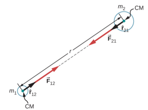
These equal but opposite forces reflect Newton’s third law, which we discussed earlier. Note that strictly speaking, Equation \ref{13.1} applies to point masses—all the mass is located at one point. But it applies equally to any spherically symmetric objects, where r is the distance between the centers of mass of those objects. In many cases, it works reasonably well for nonsymmetrical objects, if their separation is large compared to their size, and we take r to be the distance between the center of mass of each body.

Although gravity is the weakest of the four fundamental forces of nature, its attractive nature is what holds us to Earth, causes the planets to orbit the Sun and the Sun to orbit our galaxy, and binds galaxies into clusters, ranging from a few to millions. Gravity is the force that forms the Universe.

Example \(\PageIndex{1}\): A Collision in Orbit

Consider two nearly spherical Soyuz payload vehicles, in orbit about Earth, each with mass 9000 kg and diameter 4.0 m. They are initially at rest relative to each other, 10.0 m from center to center. Determine the gravitational force between them and their initial acceleration. Estimate how long it takes for them to drift together, and how fast they are moving upon impact.

Strategy

We use Newton’s law of gravitation to determine the force between them and then use Newton’s second law to find the acceleration of each. For the estimate, we assume this acceleration is constant, and we use the constant-acceleration equations from Motion along a Straight Line to find the time and speed of the collision.

Solution

The magnitude of the force is

\[|\vec{F}_{12}| = F_{12} = G \frac{m_{1} m_{2}}{r^{2}} = (6.67 \times 10^{-11}\; N\; \cdotp m^{2}/kg^{2}) \frac{(9000\; kg)(9000\; kg)}{(10\; m)^{2}} = 5.4 \times 10^{-5}\; N \ldotp\]

The initial acceleration of each payload is

\[a = \frac{F}{m} = \frac{5.4 \times 10^{-5}\; N}{9000\; kg} = 6.0 \times 10^{-9}\; m/s^{2} \ldotp\]

The vehicles are 4.0 m in diameter, so the vehicles move from 10.0 m to 4.0 m apart, or a distance of 3.0 m each. A similar calculation to that above, for when the vehicles are 4.0 m apart, yields an acceleration of 3.8 x 10⁻⁸ m/s², and the average of these two values is 2.2 x 10⁻⁸ m/s². If we assume a constant acceleration of this value and they start from rest, then the vehicles collide with speed given by

\[v^{2} = v_{0}^{2} + 2a (x - x_{0}),\; where\; v_{0} = 0,\]

so

\[v = \sqrt{2(2.2 \times 10^{-9}\; N)(3.0\; m)} = 3.6 \times 10^{-4}\; m/s \ldotp\]

We use v = v₀ + at to find t = v/a = 1.7 x 10⁴ s or about 4.6 hours.

Significance

These calculations—including the initial force—are only estimates, as the vehicles are probably not spherically symmetrical. But you can see that the force is incredibly small. Astronauts must tether themselves when doing work outside even the massive International Space Station (ISS), as in Figure \(\PageIndex{3}\), because the gravitational attraction cannot save them from even the smallest push away from the station.

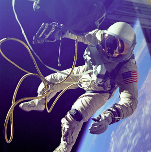
Figure \(\PageIndex{3}\): This photo shows Ed White tethered to the Space Shuttle during a spacewalk. (credit: NASA)

The effect of gravity between two objects with masses on the order of these space vehicles is indeed small. Yet, the effect of gravity on you from Earth is significant enough that a fall into Earth of only a few feet can be dangerous. We examine the force of gravity near Earth’s surface in the next section.

Example \(\PageIndex{2}\): Attraction between Galaxies

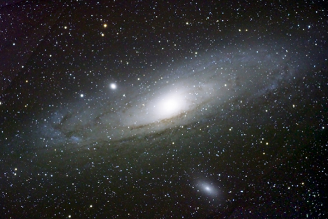
Find the acceleration of our galaxy, the Milky Way, due to the nearest comparably sized galaxy, the Andromeda galaxy (Figure \(\PageIndex{4}\)). The approximate mass of each galaxy is 800 billion solar masses (a solar mass is the mass of our Sun), and they are separated by 2.5 million light-years. (Note that the mass of Andromeda is not so well known but is believed to be slightly larger than our galaxy.) Each galaxy has a diameter of roughly 100,000 light-years (1 light-year = 9.5 x 10¹⁵ m) .

Figure \(\PageIndex{4}\): Galaxies interact gravitationally over immense distances. The Andromeda galaxy is the nearest spiral galaxy to the Milky Way, and they will eventually collide. (credit: Boris Štromar)

Strategy

As in the preceding example, we use Newton’s law of gravitation to determine the force between them and then use Newton’s second law to find the acceleration of the Milky Way. We can consider the galaxies to be point masses, since their sizes are about 25 times smaller than their separation. The mass of the Sun (see Appendix D) is 2.0 x 10³⁰ kg and a light-year is the distance light travels in one year, 9.5 x 10¹⁵ m.

Solution

The magnitude of the force is

\[F_{12} = G \frac{m_{1} m_{2}}{r^{2}} = (6.67 \times 10^{-11}\; N\; \cdotp m^{2}/kg^{2}) \frac{[(800 \times 10^{9})(2.0 \times 10^{30}\; kg)]^{2}}{[(2.5 \times 10^{6})(9.5 \times 10^{15}\; m)]^{2}} = 3.0 \times 10^{29}\; N \ldotp\]

The acceleration of the Milky Way is

\[a = \frac{F}{m} = \frac{3.0 \times 10^{29}\; N}{(800 \times 10^{9})(2.0 \times 10^{30}\; kg)} = 1.9 \times 10^{-13}\; m/s^{2} \ldotp\]

Significance

Does this value of acceleration seem astoundingly small? If they start from rest, then they would accelerate directly toward each other, “colliding” at their center of mass. Let’s estimate the time for this to happen. The initial acceleration is ~10⁻¹³ m/s², so using v = at , we see that it would take ~10¹³ s for each galaxy to reach a speed of 1.0 m/s, and they would be only ~0.5 x 10¹³ m closer. That is nine orders of magnitude smaller than the initial distance between them. In reality, such motions are rarely simple. These two galaxies, along with about 50 other smaller galaxies, are all gravitationally bound into our local cluster. Our local cluster is gravitationally bound to other clusters in what is called a supercluster. All of this is part of the great cosmic dance that results from gravitation, as shown in Figure \(\PageIndex{5}\).

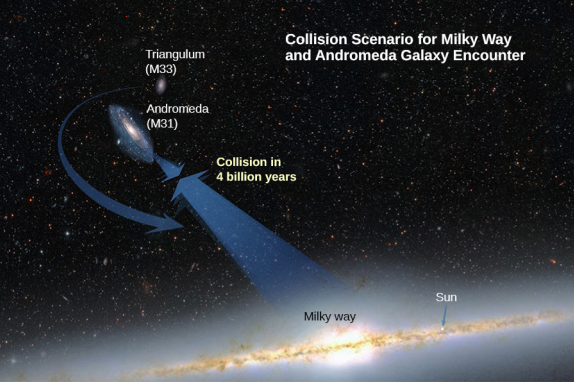
Figure \(\PageIndex{5}\): Based on the results of this example, plus what astronomers have observed elsewhere in the Universe, our galaxy will collide with the Andromeda Galaxy in about 4 billion years. (credit: NASA)

Weight - The gravitational force at the surface of the Earth

Recall that the acceleration of a free-falling object near Earth’s surface is approximately g = 9.80 m/s². The force causing this acceleration is called the weight of the object, and from Newton’s second law, it has the value mg. This weight is present regardless of whether the object is in free fall. We now know that this force is the gravitational force between the object and Earth. If we substitute mg for the magnitude of \(\vec{F}_{12}\) in Newton’s law of universal gravitation, m for m₁, and M_E for m₂, we obtain the scalar equation

\[ m g = G \frac{m M_{E}}{r^{2}} \ldotp \label{13.2}\]

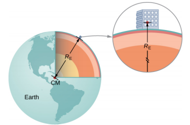
where r is the distance between the centers of mass of the object and Earth. The average radius of Earth is about 6370 km. Hence, for objects within a few kilometers of Earth’s surface, we can take \(r = R_E\) (Figure \(\PageIndex{1}\)). The mass m of the object cancels, leaving

\[g = G \frac{M_{E}}{r^{2}} \ldotp \label{13.3}\]

This explains why all masses free fall with the same acceleration. We have ignored the fact that Earth also accelerates toward the falling object, but that is acceptable as long as the mass of Earth is much larger than that of the object.

Figure \(\PageIndex{1}\): We can take the distance between the centers of mass of Earth and an object on its surface to be the radius of Earth, provided that its size is much less than the radius of Earth.

Example \(\PageIndex{1}\): Masses of Earth and Moon

Have you ever wondered how we know the mass of Earth? We certainly can’t place it on a scale. The values of g and the radius of Earth were measured with reasonable accuracy centuries ago.

1. Use the standard values of g, R_E, and Equation \ref{13.2} to find the mass of Earth.
2. Estimate the value of g on the Moon. Use the fact that the Moon has a radius of about 1700 km (a value of this accuracy was determined many centuries ago) and assume it has the same average density as Earth, 5500 kg/m³.

Strategy

With the known values of g and R_E, we can use Equation \ref{13.2} to find M_E. For the Moon, we use the assumption of equal average density to determine the mass from a ratio of the volumes of Earth and the Moon.

Solution

1. Rearranging Equation \ref{13.2}, we have \(M_{E} = \frac{g R_{E}^{2}}{G} = \frac{(9.80\; m/s^{2})(6.37 \times 10^{6}\; m)^{2}}{6.67 \times 10^{-11}\; N\; \cdotp m^{2}/kg^{2}} = 5.95 \times 10^{24}\; kg \ldotp\)
2. The volume of a sphere is proportional to the radius cubed, so a simple ratio gives us \(\frac{M_{M}}{M_{E}} = \frac{R_{M}^{3}}{R_{E}^{3}} \rightarrow M_{M} = \left(\dfrac{(1.7 \times 10^{6}\; m)^{3}}{(6.37 \times 10^{6}\; m)^{3}}\right) (5.95 \times 10^{24}\; kg) = 1.1 \times 10^{23}\; kg \ldotp\) We now use Equation \ref{13.2}. \(g_{M} = G \frac{M_{M}}{r_{M}^{2}} = (6.67 \times 10^{-11}\; N\; \cdotp m^{2}/kg^{2}) \left(\dfrac{1.1 \times 10^{23}\; kg}{(1.7 \times 10^{6}\; m)^{2}}\right) = 2.5\; m/s^{2}\)

Significance

As soon as Cavendish determined the value of G in 1798, the mass of Earth could be calculated. (In fact, that was the ultimate purpose of Cavendish’s experiment in the first place.) The value we calculated for g of the Moon is incorrect. The average density of the Moon is actually only 3340 kg/m³ and g = 1.6 m/s² at the surface. Newton attempted to measure the mass of the Moon by comparing the effect of the Sun on Earth’s ocean tides compared to that of the Moon. His value was a factor of two too small. The most accurate values for g and the mass of the Moon come from tracking the motion of spacecraft that have orbited the Moon. But the mass of the Moon can actually be determined accurately without going to the Moon. Earth and the Moon orbit about a common center of mass, and careful astronomical measurements can determine that location. The ratio of the Moon’s mass to Earth’s is the ratio of [the distance from the common center of mass to the Moon’s center] to [the distance from the common center of mass to Earth’s center].

Later in this section, we will see that the mass of other astronomical bodies also can be determined by the period of small satellites orbiting them. But until Cavendish determined the value of G, the masses of all these bodies were unknown.

Example \(\PageIndex{2}\): Gravity above Earth’s Surface

What is the value of g 400 km above Earth’s surface, where the International Space Station is in orbit?

Solution

Using the value of M_E and noting the radius is r = R_E + 400 km, we use Equation \ref{13.2} to find g. From Equation \ref{13.2} we have

\[g = G \frac{M_{E}}{r^{2}} = (6.67 \times 10^{-11}\; N\; \cdotp m^{2}/kg^{2}) \left(\dfrac{5.96 \times 10^{24}\; kg}{(6.37 \times 10^{6} + 400 \times 10^{3}\; m)^{2}}\right) = 8.67\; m/s^{2} \ldotp\]

Significance

We often see video of astronauts in space stations, apparently weightless. But clearly, the force of gravity is acting on them. Comparing the value of g we just calculated to that on Earth (9.80 m/s²) , we see that the astronauts in the International Space Station still have 88% of their weight. They only appear to be weightless because they are in free fall. We will come back to this in Satellite Orbits and Energy.

Acceleration due to gravity g varies slightly over the surface of Earth, so the weight of an object depends on its location and is not an intrinsic property of the object. Weight varies dramatically if we leave Earth’s surface. On the Moon, for example, acceleration due to gravity is only 1.67 m/s². A 1.0-kg mass thus has a weight of 9.8 N on Earth and only about 1.7 N on the Moon.

The broadest definition of weight in this sense is that the weight of an object is the gravitational force on it from the nearest large body, such as Earth, the Moon, or the Sun. This is the most common and useful definition of weight in physics. It differs dramatically, however, from the definition of weight used by NASA and the popular media in relation to space travel and exploration. When they speak of “weightlessness” and “microgravity,” they are referring to the phenomenon we call “free fall” in physics. We use the preceding definition of weight, force \(\vec{w}\) due to gravity acting on an object of mass m, and we make careful distinctions between free fall and actual weightlessness.

Be aware that weight and mass are different physical quantities, although they are closely related. Mass is an intrinsic property of an object: It is a quantity of matter. The quantity or amount of matter of an object is determined by the numbers of atoms and molecules of various types it contains. Because these numbers do not vary, in Newtonian physics, mass does not vary; therefore, its response to an applied force does not vary. In contrast, weight is the gravitational force acting on an object, so it does vary depending on gravity. For example, a person closer to the center of Earth, at a low elevation such as New Orleans, weighs slightly more than a person who is located in the higher elevation of Denver, even though they may have the same mass.

Defintion: Weight

The gravitational force on a mass is its weight. We can write this in vector form, where \(\vec{w}\) is weight and m is mass, as

\[\vec{w} = m \vec{g} \ldotp \label{5.8}\]

In scalar form, we can write

\[w = mg \ldotp \label{5.9}\]

It is tempting to equate mass to weight, because most of our examples take place on Earth, where the weight of an object varies only a little with the location of the object. In addition, it is difficult to count and identify all of the atoms and molecules in an object, so mass is rarely determined in this manner. If we consider situations in which \(\vec{g}\) is a constant on Earth, we see that weight \(\vec{w}\) is directly proportional to mass m, since \(\vec{w} = m \vec{g}\), that is, the more massive an object is, the more it weighs. Operationally, the masses of objects are determined by comparison with the standard kilogram, as we discussed in Units and Measurement. But by comparing an object on Earth with one on the Moon, we can easily see a variation in weight but not in mass. For instance, on Earth, a 5.0-kg object weighs 49 N; on the Moon, where g is 1.67 m/s², the object weighs 8.4 N. However, the mass of the object is still 5.0 kg on the Moon.

Example \(\PageIndex{3}\): Clearing a Field

A farmer is lifting some moderately heavy rocks from a field to plant crops. He lifts a stone that weighs 40.0 lb. (about 180 N). What force does he apply if the stone accelerates at a rate of 1.5 m/s²?

Strategy

We were given the weight of the stone, which we use in finding the net force on the stone. However, we also need to know its mass to apply Newton’s second law, so we must apply the equation for weight, w = mg, to determine the mass.

Solution

No forces act in the horizontal direction, so we can concentrate on vertical forces, as shown in the following free-body diagram. We label the acceleration to the side; technically, it is not part of the free-body diagram, but it helps to remind us that the object accelerates upward (so the net force is upward).

\[w = mg \nonumber \]

\[m = \frac{w}{g} = \frac{180\; N}{9.8\; m/s^{2}} = 18\; kg \nonumber\]

\[\sum F = ma \nonumber\]

\[F - w = ma \nonumber\]

\[F - 180\; N = (18\; kg)(1.5\; m/s^{2}) \nonumber\]

\[F - 180\; N = 27\; N \nonumber\]

\[F = 207\; N = 210\; N\; \text{ to two significant figures} \nonumber\]

Significance

To apply Newton’s second law as the primary equation in solving a problem, we sometimes have to rely on other equations, such as the one for weight or one of the kinematic equations, to complete the solution.

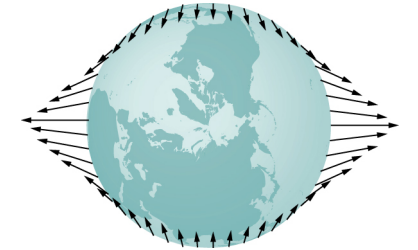
The Gravitational Field

Equation \ref{13.2} is a scalar equation, giving the magnitude of the gravitational acceleration as a function of the distance from the center of the mass that causes the acceleration. But we could have retained the vector form for the force of gravity in Equation \ref{13.1}, and written the acceleration in vector form as

\[\vec{g} = G \frac{M}{r^{2}} \hat{r} \ldotp\]

We identify the vector field represented by \(\vec{g}\) as the gravitational field caused by mass M. We can picture the field as shown Figure \(\PageIndex{2}\). The lines are directed radially inward and are symmetrically distributed about the mass.

Figure \(\PageIndex{2}\): A three-dimensional representation of the gravitational field created by mass M . Note that the lines are uniformly distributed in all directions. (The box has been added only to aid in visualization.)

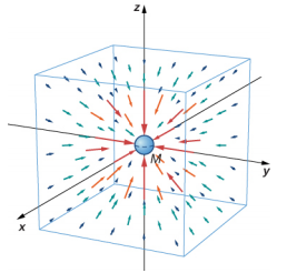
As is true for any vector field, the direction of \(\vec{g}\) is parallel to the field lines at any point. The strength of \(\vec{g}\) at any point is inversely proportional to the line spacing. Another way to state this is that the magnitude of the field in any region is proportional to the number of lines that pass through a unit surface area, effectively a density of lines. Since the lines are equally spaced in all directions, the number of lines per unit surface area at a distance r from the mass is the total number of lines divided by the surface area of a sphere of radius r, which is proportional to r 2 . Hence, this picture perfectly represents the inverse square law, in addition to indicating the direction of the field. In the field picture, we say that a mass m interacts with the gravitational field of mass M. We will use the concept of fields to great advantage in the later sections on electromagnetism.

Gravity Away from the Surface

Earlier we stated without proof that the law of gravitation applies to spherically symmetrical objects, where the mass of each body acts as if it were at the center of the body. Since Equation \ref{13.2} is derived from Equation \ref{13.1}, it is also valid for symmetrical mass distributions, but both equations are valid only for values of \(r ≥ R_E\). As we saw in Example 13.4, at 400 km above Earth’s surface, where the International Space Station orbits, the value of \(g\) is 8.67 m/s². (We will see later that this is also the centripetal acceleration of the ISS.)

For \(r < R_E\), Equation \ref{13.1} and Equation \ref{13.2} are not valid. However, we can determine g for these cases using a principle that comes from Gauss’s law, which is a powerful mathematical tool that we study in more detail later in the course. A consequence of Gauss’s law, applied to gravitation, is that only the mass within r contributes to the gravitational force. Also, that mass, just as before, can be considered to be located at the center. The gravitational effect of the mass outside r has zero net effect.

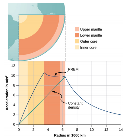
Two very interesting special cases occur. For a spherical planet with constant density, the mass within r is the density times the volume within r. This mass can be considered located at the center. Replacing M_E with only the mass within r, M = \(\rho\) x (volume of a sphere), and R_E with r, Equation \ref{13.2} becomes

\[g = G \frac{M_{E}}{R_{E}^{2}} = G \frac{\rho \left(\dfrac{4}{3} \pi r^{3}\right)}{r^{2}} = \frac{4}{3} G \rho \pi r \ldotp\]

The value of g, and hence your weight, decreases linearly as you descend down a hole to the center of the spherical planet. At the center, you are weightless, as the mass of the planet pulls equally in all directions. Actually, Earth’s density is not constant, nor is Earth solid throughout. Figure \(\PageIndex{4}\) shows the profile of \(g\) if Earth had constant density and the more likely profile based upon estimates of density derived from seismic data.

Figure \(\PageIndex{4}\): For r < RE, the value of g for the case of constant density is the straight green line. The blue line from the PREM (Preliminary Reference Earth Model) is probably closer to the actual profile for g.

The second interesting case concerns living on a spherical shell planet. This scenario has been proposed in many science fiction stories. Ignoring significant engineering issues, the shell could be constructed with a desired radius and total mass, such that g at the surface is the same as Earth’s. Can you guess what happens once you descend in an elevator to the inside of the shell, where there is no mass between you and the center? What benefits would this provide for traveling great distances from one point on the sphere to another? And finally, what effect would there be if the planet was spinning?

Tidal Forces

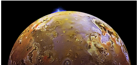
The origin of Earth’s ocean tides has been a subject of continuous investigation for over 2000 years. But the work of Newton is considered to be the beginning of the true understanding of the phenomenon. Ocean tides are the result of gravitational tidal forces. These same tidal forces are present in any astronomical body. They are responsible for the internal heat that creates the volcanic activity on Io, one of Jupiter’s moons, and the breakup of stars that get too close to black holes.

Lunar Tides

If you live on an ocean shore almost anywhere in the world, you can observe the rising and falling of the sea level about twice per day. This is caused by a combination of Earth’s rotation about its axis and the gravitational attraction of both the Moon and the Sun.

Let’s consider the effect of the Moon first. In Figure \(\PageIndex{1}\), we are looking “down” onto Earth’s North Pole. One side of Earth is closer to the Moon than the other side, by a distance equal to Earth’s diameter. Hence, the gravitational force is greater on the near side than on the far side. The magnitude at the center of Earth is between these values. This is why a tidal bulge appears on both sides of Earth.

Figure \(\PageIndex{1}\): The tidal force stretches Earth along the line between Earth and the Moon. It is the difference between the gravitational force from the far side to the near side that creates the tidal bulge on both sides of the planet. Tidal variations of the oceans are on the order of few meters; hence, this diagram is greatly exaggerated.

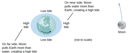
The net force on Earth causes it to orbit about the Earth-Moon center of mass, located about 1600 km below Earth’s surface along the line between Earth and the Moon. The tidal force can be viewed as the difference between the force at the center of Earth and that at any other location. In Figure \(\PageIndex{2}\), this difference is shown at sea level, where we observe the ocean tides. (Note that the change in sea level caused by these tidal forces is measured from the baseline sea level. We saw earlier that Earth bulges many kilometers at the equator due to its rotation. This defines the baseline sea level and here we consider only the much smaller tidal bulge measured from that baseline sea level.)

Figure \(\PageIndex{2}\): The tidal force is the difference between the gravitational force at the center and that elsewhere. In this figure, the tidal forces are shown at the ocean surface. These forces would diminish to zero as you approach Earth’s center.

Why does the rise and fall of the tides occur twice per day? Look again at Figure \(\PageIndex{1}\). If Earth were not rotating and the Moon was fixed, then the bulges would remain in the same location on Earth. Relative to the Moon, the bulges stay fixed—along the line connecting Earth and the Moon. But Earth rotates (in the direction shown by the blue arrow) approximately every 24 hours. In 6 hours, the near and far locations of Earth move to where the low tides are occurring, and 6 hours later, those locations are back to the high-tide position. Since the Moon also orbits Earth approximately every 28 days, and in the same direction as Earth rotates, the time between high (and low) tides is actually about 12.5 hours. The actual timing of the tides is complicated by numerous factors, the most important of which is another astronomical body—the Sun.

The Effect of the Sun on Tides

In addition to the Moon’s tidal forces on Earth’s oceans, the Sun exerts a tidal force as well. The gravitational attraction of the Sun on any object on Earth is nearly 200 times that of the Moon. However, as we show later in an example, the tidal effect of the Sun is less than that of the Moon, but a significant effect nevertheless. Depending upon the positions of the Moon and Sun relative to Earth, the net tidal effect can be amplified or attenuated.

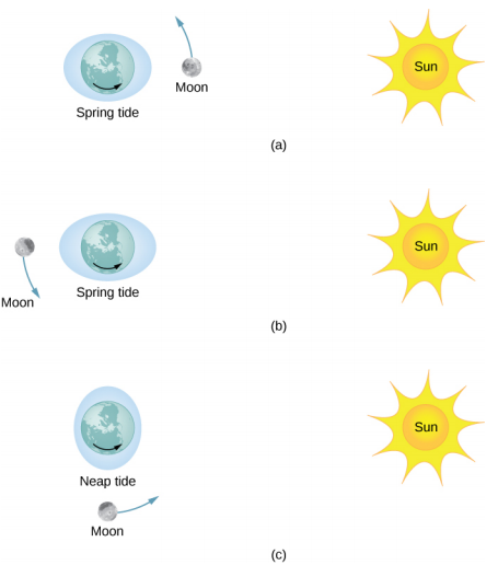
Figure \(\PageIndex{3}\) illustrates the relative positions of the Sun and the Moon that create the largest tides, called spring tides (or leap tides). During spring tides, Earth, the Moon, and the Sun are aligned and the tidal effects add. (Recall that the tidal forces cause bulges on both sides.) Figure \(\PageIndex{3c}\) shows the relative positions for the smallest tides, called neap tides. The extremes of both high and low tides are affected. Spring tides occur during the new or full moon, and neap tides occur at half-moon.

Figure \(\PageIndex{3}\): (a and b) The spring tides occur when the Sun and the Moon are aligned, whereas (c) the neap tides occur when the Sun and Moon make a right triangle with Earth. (Figure is not drawn to scale.)

The Magnitude of the Tides

With accurate data for the positions of the Moon and the Sun, the time of maximum and minimum tides at most locations on our planet can be predicted accurately. The magnitude of the tides, however, is far more complicated. The relative angles of Earth and the Moon determine spring and neap tides, but the magnitudes of these tides are affected by the distances from Earth as well. Tidal forces are greater when the distances are smaller. Both the Moon’s orbit about Earth and Earth’s orbit about the Sun are elliptical, so a spring tide is exceptionally large if it occurs when the Moon is at perigee and Earth is at perihelion. Conversely, it is relatively small if it occurs when the Moon is at apogee and Earth is at aphelion.

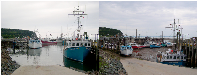
The greatest causes of tide variation are the topography of the local shoreline and the bathymetry (the profile of the depth) of the ocean floor. The range of tides due to these effects is astounding. Although ocean tides are much smaller than a meter in many places around the globe, the tides at the Bay of Fundy (Figure \(\PageIndex{4}\)), on the east coast of Canada, can be as much as 16.3 meters.

Figure \(\PageIndex{4}\): Boats in the Bay of Fundy at high and low tides. The twice-daily change in sea level creates a real challenge to the safe mooring of boats. (credit: Dylan Kereluk)

Example \(\PageIndex{1}\): Comparing Tidal Forces

Compare the Moon’s gravitational force on a 1.0-kg mass located on the near side and another on the far side of Earth. Repeat for the Sun and then compare the results to confirm that the Moon’s tidal forces are about twice that of the Sun.

Strategy

We use Newton’s law of gravitation given by Equation 13.2.1. We need the masses of the Moon and the Sun and their distances from Earth, as well as the radius of Earth. We use the astronomical data from Appendix D.

Solution

Substituting the mass of the Moon and mean distance from Earth to the Moon, we have

\[F_{12} = G \frac{m_{1} m_{2}}{r^{2}} = (6.67 \times 10^{-11}\; N\; \cdotp m^{2}/kg^{2}) \Bigg[ \frac{(1.0\; kg)(7.35 \times 10^{22}\; kg)}{(3.84 \times 10^{8} \pm 6.37 \times 10^{6}\; m)^{2}} \Bigg] \ldotp\]

In the denominator, we use the minus sign for the near side and the plus sign for the far side. The results are

\[F_{near} = 3.44 \times 10^{-5}\; N\; and\; F_{far} = 3.22 \times 10^{-5}\; N \ldotp\]

The Moon’s gravitational force is nearly 7% higher at the near side of Earth than at the far side, but both forces are much less than that of Earth itself on the 1.0-kg mass. Nevertheless, this small difference creates the tides. We now repeat the problem, but substitute the mass of the Sun and the mean distance between the Earth and Sun. The results are

\[F_{near} = 5.89975 \times 10^{-3}\; N\; and\; F_{far} = 5.89874 \times 10^{-3}\; N \ldotp\]

We have to keep six significant digits since we wish to compare the difference between them to the difference for the Moon. (Although we can’t justify the absolute value to this accuracy, since all values in the calculation are the same except the distances, the accuracy in the difference is still valid to three digits.) The difference between the near and far forces on a 1.0-kg mass due to the Moon is

\[F_{near} = (3.44 \times 10^{-5}\; N) - (3.22 \times 10^{-5}\; N) = 0.22 \times 10^{-5}\; N,\]

whereas the difference for the Sun is

\[F_{near} - F_{far} = (5.89975 \times 10^{-3}\; N) - (5.89874 \times 10^{-3}\; N) = 0.101 \times 10^{-5}\; N \ldotp\]

Note that a more proper approach is to write the difference in the two forces with the difference between the near and far distances explicitly expressed. With just a bit of algebra we can show that

\[F_{tidal} = \frac{GMm}{r_{1}^{2}} - \frac{GMm}{r_{2}^{2}} = GMm \left(\dfrac{(r_{2} - r_{1})(r_{2} + r_{1})}{r_{1}^{2} r_{2}^{2}} \right) \ldotp\]

where r₁ and r₂ are the same to three significant digits, but their difference (r₂ − r₁), equal to the diameter of Earth, is also known to three significant digits. The results of the calculation are the same. This approach would be necessary if the number of significant digits needed exceeds that available on your calculator or computer.

Significance

Note that the forces exerted by the Sun are nearly 200 times greater than the forces exerted by the Moon. But the difference in those forces for the Sun is half that for the Moon. This is the nature of tidal forces. The Moon has a greater tidal effect because the fractional change in distance from the near side to the far side is so much greater for the Moon than it is for the Sun.

Other Tidal Effects

Tidal forces exist between any two bodies. The effect stretches the bodies along the line between their centers. Although the tidal effect on Earth’s seas is observable on a daily basis, long-term consequences cannot be observed so easily. One consequence is the dissipation of rotational energy due to friction during flexure of the bodies themselves. Earth’s rotation rate is slowing down as the tidal forces transfer rotational energy into heat. The other effect, related to this dissipation and conservation of angular momentum, is called “locking” or tidal synchronization. It has already happened to most moons in our solar system, including Earth’s Moon. The Moon keeps one face toward Earth—its rotation rate has locked into the orbital rate about Earth. The same process is happening to Earth, and eventually it will keep one face toward the Moon. If that does happen, we would no longer see tides, as the tidal bulge would remain in the same place on Earth, and half the planet would never see the Moon. However, this locking will take many billions of years, perhaps not before our Sun expires.

One of the more dramatic example of tidal effects is found on Io, one of Jupiter’s moons. In 1979, the Voyager spacecraft sent back dramatic images of volcanic activity on Io. It is the only other astronomical body in our solar system on which we have found such activity. Figure \(\PageIndex{5}\) shows a more recent picture of Io taken by the New Horizons spacecraft on its way to Pluto, while using a gravity assist from Jupiter.

Figure \(\PageIndex{5}\): Dramatic evidence of tidal forces can be seen on Io. The eruption seen in blue is due to the internal heat created by the tidal forces exerted on Io by Jupiter.

For some stars, the effect of tidal forces can be catastrophic. The tidal forces in very close binary systems can be strong enough to rip matter from one star to the other, once the tidal forces exceed the cohesive self-gravitational forces that hold the stars together. This effect can be seen in normal stars that orbit nearby compact stars, such as neutron stars or black holes. Figure \(\PageIndex{6}\) shows an artist’s rendition of this process. As matter falls into the compact star, it forms an accretion disc that becomes super-heated and radiates in the X-ray spectrum.

Figure \(\PageIndex{6}\): Tidal forces from a compact object can tear matter away from an orbiting star. In addition to the accretion disc orbiting the compact object, material is often ejected along relativistic jets as shown. (credit: modification of work by European Southern Observatory (ESO))

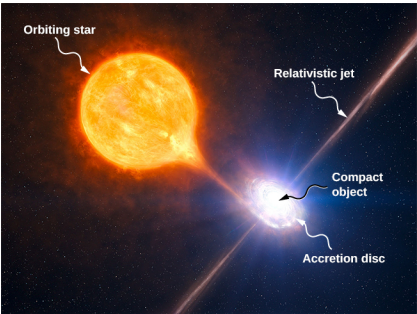
The energy output of these binary systems can exceed the typical output of thousands of stars. Another example might be a quasar. Quasars are very distant and immensely bright objects, often exceeding the energy output of entire galaxies. It is the general consensus among astronomers that they are, in fact, massive black holes producing radiant energy as matter that has been tidally ripped from nearby stars falls into them.

Einstein's Theory of Gravity

Newton’s law of universal gravitation accurately predicts much of what we see within our solar system. Indeed, only Newton’s laws have been needed to accurately send every space vehicle on its journey. The paths of Earth-crossing asteroids, and most other celestial objects, can be accurately determined solely with Newton’s laws. Nevertheless, many phenomena have shown a discrepancy from what Newton’s laws predict, including the orbit of Mercury and the effect that gravity has on light. In this section, we examine a different way of envisioning gravitation.

A Revolution in Perspective

In 1905, Albert Einstein published his theory of special relativity. This theory is discussed in great detail in Relativity so we say only a few words here. In this theory, no motion can exceed the speed of light—it is the speed limit of the Universe. This simple fact has been verified in countless experiments. However, it has incredible consequences—space and time are no longer absolute. Two people moving relative to one another do not agree on the length of objects or the passage of time. Almost all of the mechanics you learned in previous chapters, while remarkably accurate even for speeds of many thousands of miles per second, begin to fail when approaching the speed of light.

This speed limit on the Universe was also a challenge to the inherent assumption in Newton’s law of gravitation that gravity is an action-at-a-distance force. That is, without physical contact, any change in the position of one mass is instantly communicated to all other masses. This assumption does not come from any first principle, as Newton’s theory simply does not address the question. (The same was believed of electromagnetic forces, as well. It is fair to say that most scientists were not completely comfortable with the action-at-a-distance concept.)

A second assumption also appears in Newton’s law of gravitation Equation 13.2.1. The masses are assumed to be exactly the same as those used in Newton’s second law, \(\vec{F}\) = m\(\vec{a}\). We made that assumption in many of our derivations in this chapter. Again, there is no underlying principle that this must be, but experimental results are consistent with this assumption. In Einstein’s subsequent theory of general relativity (1916), both of these issues were addressed. His theory was a theory of space-time geometry and how mass (and acceleration) distort and interact with that space-time. It was not a theory of gravitational forces. The mathematics of the general theory is beyond the scope of this text, but we can look at some underlying principles and their consequences.

The Principle of Equivalence

Einstein came to his general theory in part by wondering why someone who was free falling did not feel his or her weight. Indeed, it is common to speak of astronauts orbiting Earth as being weightless, despite the fact that Earth’s gravity is still quite strong there. In Einstein’s general theory, there is no difference between free fall and being weightless. This is called the principle of equivalence. The equally surprising corollary to this is that there is no difference between a uniform gravitational field and a uniform acceleration in the absence of gravity. Let’s focus on this last statement. Although a perfectly uniform gravitational field is not feasible, we can approximate it very well.

Within a reasonably sized laboratory on Earth, the gravitational field \(\vec{g}\) is essentially uniform. The corollary states that any physical experiments performed there have the identical results as those done in a laboratory accelerating at \(\vec{a} = \vec{g}\) in deep space, well away from all other masses. Figure \(\PageIndex{1}\) illustrates the concept.

Figure \(\PageIndex{1}\): According to the principle of equivalence, the results of all experiments performed in a laboratory in a uniform gravitational field are identical to the results of the same experiments performed in a uniformly accelerating laboratory.

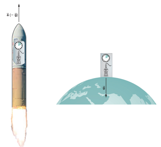
How can these two apparently fundamentally different situations be the same? The answer is that gravitation is not a force between two objects but is the result of each object responding to the effect that the other has on the space-time surrounding it. A uniform gravitational field and a uniform acceleration have exactly the same effect on space-time.

A Geometric Theory of Gravity

Euclidian geometry assumes a “flat” space in which, among the most commonly known attributes, a straight line is the shortest distance between two points, the sum of the angles of all triangles must be 180 degrees, and parallel lines never intersect. Non-Euclidean geometry was not seriously investigated until the nineteenth century, so it is not surprising that Euclidean space is inherently assumed in all of Newton’s laws.

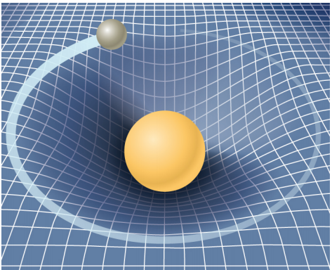
The general theory of relativity challenges this long-held assumption. Only empty space is flat. The presence of mass—or energy, since relativity does not distinguish between the two—distorts or curves space and time, or space-time, around it. The motion of any other mass is simply a response to this curved space-time. Figure \(\PageIndex{2}\) is a two-dimensional representation of a smaller mass orbiting in response to the distorted space created by the presence of a larger mass. In a more precise but confusing picture, we would also see space distorted by the orbiting mass, and both masses would be in motion in response to the total distortion of space. Note that the figure is a representation to help visualize the concept. These are distortions in our three-dimensional space and time. We do not see them as we would a dimple on a ball. We see the distortion only by careful measurements of the motion of objects and light as they move through space.

Figure \(\PageIndex{2}\): A smaller mass orbiting in the distorted space-time of a larger mass. In fact, all mass or energy distorts space-time.

For weak gravitational fields, the results of general relativity do not differ significantly from Newton’s law of gravitation. But for intense gravitational fields, the results diverge, and general relativity has been shown to predict the correct results. Even in our Sun’s relatively weak gravitational field at the distance of Mercury’s orbit, we can observe the effect. Starting in the mid-1800s, Mercury’s elliptical orbit has been carefully measured. However, although it is elliptical, its motion is complicated by the fact that the perihelion position of the ellipse slowly advances. Most of the advance is due to the gravitational pull of other planets, but a small portion of that advancement could not be accounted for by Newton’s law. At one time, there was even a search for a “companion” planet that would explain the discrepancy. But general relativity correctly predicts the measurements. Since then, many measurements, such as the deflection of light of distant objects by the Sun, have verified that general relativity correctly predicts the observations.

We close this discussion with one final comment. We have often referred to distortions of space-time or distortions in both space and time. In both special and general relativity, the dimension of time has equal footing with each spatial dimension (differing in its place in both theories only by an ultimately unimportant scaling factor). Near a very large mass, not only is the nearby space “stretched out,” but time is dilated or “slowed.” We discuss these effects more in the next section.

Black Holes

Einstein’s theory of gravitation is expressed in one deceptively simple-looking tensor equation (tensors are a generalization of scalars and vectors), which expresses how a mass determines the curvature of space-time around it. The solutions to that equation yield one of the most fascinating predictions: the black hole. The prediction is that if an object is sufficiently dense, it will collapse in upon itself and be surrounded by an event horizon from which nothing can escape. The name “black hole,” which was coined by astronomer John Wheeler in 1969, refers to the fact that light cannot escape such an object. Karl Schwarzschild was the first person to note this phenomenon in 1916, but at that time, it was considered mostly to be a mathematical curiosity.

Surprisingly, the idea of a massive body from which light cannot escape dates back to the late 1700s. Independently, John Michell and Pierre Simon Laplace used Newton’s law of gravitation to show that light leaving the surface of a star with enough mass could not escape. Their work was based on the fact that the speed of light had been measured by Ole Roemer in 1676. He noted discrepancies in the data for the orbital period of the moon Io about Jupiter. Roemer realized that the difference arose from the relative positions of Earth and Jupiter at different times and that he could find the speed of light from that difference. Michell and Laplace both realized that since light had a finite speed, there could be a star massive enough that the escape speed from its surface could exceed that speed. Hence, light always would fall back to the star. Oddly, observers far enough away from the very largest stars would not be able to see them, yet they could see a smaller star from the same distance.

Recall that in Gravitational Potential Energy and Total Energy, we found that the escape speed, given by \(v_{\mathrm{esc}}=\sqrt{\frac{2 G M}{R}}\), is independent of the mass of the object escaping. Even though the nature of light was not fully understood at the time, the mass of light, if it had any, was not relevant. Hence, this equation should be valid for light. Substituting c, the speed of light, for the escape velocity, we have

\[v_{esc} = c = \sqrt{\dfrac{2GM}{R}} \ldotp\]

Thus, we only need values for R and M such that the escape velocity exceeds c, and then light will not be able to escape. Michell posited that if a star had the density of our Sun and a radius that extended just beyond the orbit of Mars, then light would not be able to escape from its surface. He also conjectured that we would still be able to detect such a star from the gravitational effect it would have on objects around it. This was an insightful conclusion, as this is precisely how we infer the existence of such objects today. While we have yet to, and may never, visit a black hole, the circumstantial evidence for them has become so compelling that few astronomers doubt their existence.

Before we examine some of that evidence, we turn our attention back to Schwarzschild’s solution to the tensor equation from general relativity. In that solution arises a critical radius, now called the Schwarzschild radius (R_S). For any mass M, if that mass were compressed to the extent that its radius becomes less than the Schwarzschild radius, then the mass will collapse to a singularity, and anything that passes inside that radius cannot escape. Once inside R_S, the arrow of time takes all things to the singularity. (In a broad mathematical sense, a singularity is where the value of a function goes to infinity. In this case, it is a point in space of zero volume with a finite mass. Hence, the mass density and gravitational energy become infinite.) The Schwarzschild radius is given by

\[R_{S} = \dfrac{2GM}{c^{2}} \ldotp \label{13.12}\]

If you look at our escape velocity equation with v_esc = c, you will notice that it gives precisely this result. But that is merely a fortuitous accident caused by several incorrect assumptions. One of these assumptions is the use of the incorrect classical expression for the kinetic energy for light. Just how dense does an object have to be in order to turn into a black hole?

Example \(\PageIndex{1}\): Calculating the Schwarzschild Radius

Calculate the Schwarzschild radius for both the Sun and Earth. Compare the density of the nucleus of an atom to the density required to compress Earth’s mass uniformly to its Schwarzschild radius. The density of a nucleus is about 2.3 x 10¹⁷ kg/m³.

Strategy

We use Equation \ref{13.12} for this calculation. We need only the masses of Earth and the Sun, which we obtain from the astronomical data given in Appendix D.

Solution

Substituting the mass of the Sun, we have

\[R_{S} = \dfrac{2GM}{c^{2}} = \dfrac{2(6.67 \times 10^{-11}\; N\; \cdotp m^{2}/kg^{2})(1.99 \times 10^{30}\; kg)}{(3.0 \times 10^{8}\; m/s)^{2}} = 2.95 \times 10^{3}\; m \ldotp\]

This is a diameter of only about 6 km. If we use the mass of Earth, we get R_S = 8.85 x 10⁻³ m. This is a diameter of less than 2 cm! If we pack Earth’s mass into a sphere with the radius R_S = 8.85 x 10⁻³ m, we get a density of

\[\rho = \dfrac{mass}{volume} = \dfrac{5.97 \times 10^{24}\; kg}{\dfrac{4}{3} \pi (8.85 \times 10^{-3}\; m)^{3}} = 2.06 \times 10^{30}\; kg/m^{3} \ldotp\]

Significance

A neutron star is the most compact object known—outside of a black hole itself. The neutron star is composed of neutrons, with the density of an atomic nucleus, and, like many black holes, is believed to be the remnant of a supernova—a star that explodes at the end of its lifetime. To create a black hole from Earth, we would have to compress it to a density thirteen orders of magnitude greater than that of a neutron star. This process would require unimaginable force. There is no known mechanism that could cause an Earth-sized object to become a black hole. For the Sun, you should be able to show that it would have to be compressed to a density only about 80 times that of a nucleus. (Note: Once the mass is compressed within its Schwarzschild radius, general relativity dictates that it will collapse to a singularity. These calculations merely show the density we must achieve to initiate that collapse.)

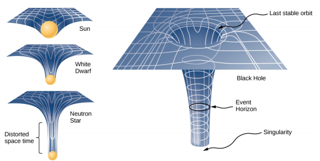
The Event Horizon

The Schwarzschild radius is also called the event horizon of a black hole. We noted that both space and time are stretched near massive objects, such as black holes. Figure \(\PageIndex{3}\) illustrates that effect on space. The distortion caused by our Sun is actually quite small, and the diagram is exaggerated for clarity. Consider the neutron star, described in Example \(\PageIndex{1}\). Although the distortion of space-time at the surface of a neutron star is very high, the radius is still larger than its Schwarzschild radius. Objects could still escape from its surface.

However, if a neutron star gains additional mass, it would eventually collapse, shrinking beyond the Schwarzschild radius. Once that happens, the entire mass would be pulled, inevitably, to a singularity. In the diagram, space is stretched to infinity. Time is also stretched to infinity. As objects fall toward the event horizon, we see them approaching ever more slowly, but never reaching the event horizon. As outside observers, we never see objects pass through the event horizon—effectively, time is stretched to a stop.

Simulation

Visit this site to view an animated example of these spatial distortions.

Figure \(\PageIndex{3}\): The space distortion becomes more noticeable around increasingly larger masses. Once the mass density reaches a critical level, a black hole forms and the fabric of space-time is torn. The curvature of space is greatest at the surface of each of the first three objects shown and is finite. The curvature then decreases (not shown) to zero as you move to the center of the object. But the black hole is different. The curvature becomes infinite: The surface has collapsed to a singularity, and the cone extends to infinity. (Note: These diagrams are not to any scale.)

The evidence for black holes

Not until the 1960s, when the first neutron star was discovered, did interest in the existence of black holes become renewed. Evidence for black holes is based upon several types of observations, such as radiation analysis of X-ray binaries, gravitational lensing of the light from distant galaxies, and the motion of visible objects around invisible partners. We will focus on these later observations as they relate to what we have learned in this chapter. Although light cannot escape from a black hole for us to see, we can nevertheless see the gravitational effect of the black hole on surrounding masses.

The closest, and perhaps most dramatic, evidence for a black hole is at the center of our Milky Way galaxy. The UCLA Galactic Group, using data obtained by the W. M. Keck telescopes, has determined the orbits of several stars near the center of our galaxy. Some of that data is shown in Figure \(\PageIndex{4}\). The orbits of two stars are highlighted. From measurements of the periods and sizes of their orbits, it is estimated that they are orbiting a mass of approximately 4 million solar masses. Note that the mass must reside in the region created by the intersection of the ellipses of the stars. The region in which that mass must reside would fit inside the orbit of Mercury—yet nothing is seen there in the visible spectrum.

Figure \(\PageIndex{4}\): Paths of stars orbiting about a mass at the center of our Milky Way galaxy. From their motion, it is estimated that a black hole of about 4 million solar masses resides at the center. (credit: UCLA Galactic Center Group – W.M. Keck Observatory Laser Team)

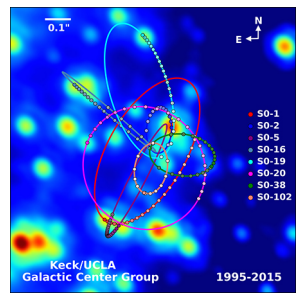
The physics of stellar creation and evolution is well established. The ultimate source of energy that makes stars shine is the self-gravitational energy that triggers fusion. The general behavior is that the more massive a star, the brighter it shines and the shorter it lives. The logical inference is that a mass that is 4 million times the mass of our Sun, confined to a very small region, and that cannot be seen, has no viable interpretation other than a black hole. Extragalactic observations strongly suggest that black holes are common at the center of galaxies.

Dark Matter

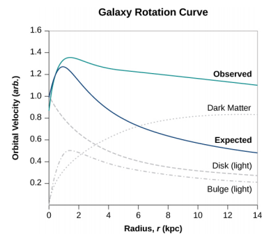
Stars orbiting near the very heart of our galaxy provide strong evidence for a black hole there, but the orbits of stars far from the center suggest another intriguing phenomenon that is observed indirectly as well. Recall from Gravitation Near Earth’s Surface that we can consider the mass for spherical objects to be located at a point at the center for calculating their gravitational effects on other masses. Similarly, we can treat the total mass that lies within the orbit of any star in our galaxy as being located at the center of the Milky Way disc. We can estimate that mass from counting the visible stars and include in our estimate the mass of the black hole at the center as well.

But when we do that, we find the orbital speed of the stars is far too fast to be caused by that amount of matter. Figure \(\PageIndex{5}\) shows the orbital velocities of stars as a function of their distance from the center of the Milky Way. The blue line represents the velocities we would expect from our estimates of the mass, whereas the green curve is what we get from direct measurements. Apparently, there is a lot of matter we don’t see, estimated to be about five times as much as what we do see, so it has been dubbed dark matter. Furthermore, the velocity profile does not follow what we expect from the observed distribution of visible stars. Not only is the estimate of the total mass inconsistent with the data, but the expected distribution is inconsistent as well. And this phenomenon is not restricted to our galaxy, but seems to be a feature of all galaxies. In fact, the issue was first noted in the 1930s when galaxies within clusters were measured to be orbiting about the center of mass of those clusters faster than they should based upon visible mass estimates.

Figure \(\PageIndex{5}\): The blue curve shows the expected orbital velocity of stars in the Milky Way based upon the visible stars we can see. The green curve shows that the actually velocities are higher, suggesting additional matter that cannot be seen. (credit: modification of work by Matthew Newby)

There are two prevailing ideas of what this matter could be—WIMPs and MACHOs. WIMPs stands for weakly interacting massive particles. These particles (neutrinos are one example) interact very weakly with ordinary matter and, hence, are very difficult to detect directly. MACHOs stands for massive compact halo objects, which are composed of ordinary baryonic matter, such as neutrons and protons. There are unresolved issues with both of these ideas, and far more research will be needed to solve the mystery.