21.1: Banking

Example \(\PageIndex{1}\): Going around a banked curve

Roadway engineers often bank a curve, especially if it is a very tight turn, so the cars will not have to rely on friction alone to provide the required centripetal force. The picture shows a car going around such a curve, which we can model as an arc of a circle of radius \(r\). In terms of \(r\), the bank angle \(\theta\), and the coefficient of static friction, find the maximum safe speed around the curve.

Figure \(\PageIndex{2}\): A car going around a banked curve (sketch and free-body diagram). The center of the circle is towards the right.

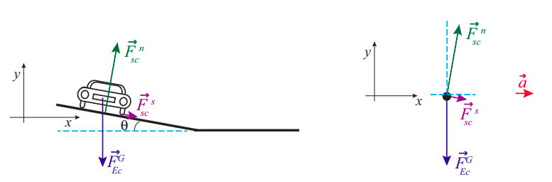
The figure shows the appropriate choice of axes for this problem. The criterion is, again, to choose the axes so that one of them will coincide with the direction of the acceleration. In this case, the acceleration is all centripetal, that is to say, pointing, horizontally, towards the center of the circle on which the car is traveling.

It may seem strange to see the force of static friction pointing down the slope, but recall that for a car turning on a flat surface it would have been pointing inwards (towards the center of the circle), so this is the natural extension of that. In general, you should always try to imagine which way the object would slide if friction disappeared altogether: \(\vec F^s\) must point in the direction opposite that. Thus, for a car traveling at a reasonable speed, the direction in which it would skid is up the slope, and that means \(\vec F^s\) must point down the slope. But, for a car just sitting still on the tilted road, \(\vec F^s\) must point upwards, and we shall see in a moment that in general there is a minimum velocity required for the force of static friction to point in the direction we have chosen.

Apart from this, the main difference with the flat surface case is that now the normal force has a component along the direction of the acceleration, so it helps to keep the car moving in a circle. On the other hand, note that we now lose (for centripetal purposes) a little bit of the friction force, since it is pointing slightly downwards. This, however, is more than compensated for by the fact that the normal force is greater now than it would be for a flat surface, since the car is now, so to speak, “driving into” the road somewhat.

The dashed blue lines in the free-body diagram are meant to indicate that the angle \(\theta\) of the bank is also the angle between the normal force and the positive \(y\) axis, as well as the angle that \(\vec F^s\) makes below the positive \(x\) axis. It follows that the components of these two forces along the axes shown are:

\begin{align}
&F_{x}^{n}=F^{n} \sin \theta \nonumber \\
&F_{y}^{n}=F^{n} \cos \theta \label{eq:8.55}
\end{align}

and

\begin{align}
&F_{x}^{s}=F^{s} \cos \theta \nonumber \\
&F_{y}^{n}=-F^{s} \sin \theta \label{eq:8.56}
\end{align}

Our force equation in column vector form is:

\[\begin{bmatrix}F_{x}^{n}\\F_{y}^{n}\\0\end{bmatrix}+\begin{bmatrix}F_{x}^{s}\\F_{y}^{s}\\0\end{bmatrix}+\begin{bmatrix}0\\-F^{g}\\0\end{bmatrix}=\begin{bmatrix}F^{n} \sin \theta+F^{s} \cos \theta\\F^{n} \cos \theta-F^{s} \sin \theta-m g\\0\end{bmatrix} = \begin{bmatrix} \frac{m v^{2}}{r}\\0\\0 \end{bmatrix}\label{eq:8.57}\]

where I have already substituted the value of the centripetal acceleration for \(a_x\) and 0 for \(a_y\) and \(a_z\).

This shows that \(F^n = (mg + F^s \sin \theta)/ \cos \theta \) is indeed greater than just \(mg\) for this problem, and must increase as the angle \(\theta\) increases (since \(\cos \theta\) decreases with increasing \(\theta\)).

The first and second lines of Equation (\ref{eq:8.77}) form a system that needs to be solved for the two unknowns \(F^n\) and \(F^s\). The result is:

\begin{align}
&F^{n}=m g \cos \theta+\frac{m v^{2}}{r} \sin \theta \nonumber \\
&F^{s}=-m g \sin \theta+\frac{m v^{2}}{r} \cos \theta \label{eq:8.59}.
\end{align}

Note that the second equation would have \(F^s\) becoming negative if \( v^{2}<g r \tan \theta \). This means that below that speed, the force of static friction must actually point up the slope, as discussed above. We can call this particular speed, for which \(F^s\) becomes zero, \(v_{no \: friction}\):

\[ v_{\text {no friction }}=\sqrt{g r \tan \theta} \label{eq:8.60} .\]

What this means is that it is possible to arrange the banking angle so that a car going at a specific speed would not have to rely on friction at all in order to make the curve: the normal force would be just right to provide the required centripetal acceleration. A car going at that speed would not feel either pulled down or pushed up the slope. However, a car going faster than that would tend to “fly off”, and the static friction force would be required to pull it in and keep it on the curve, whereas a car moving more slowly would tend to slide down and would have to be pushed up by the friction force. Friction, therefore, provides a range of safe speeds to drive in this case, just as it did in the flat surface case.

We can calculate the maximum safe speed as we did before, recalling that we must always have \(F^{s} \leq \mu_{s} F^{n}\). Substituting Eqs. (\ref{eq:8.59}) in this expression, and solving for \(v\), we get the condition

\[ v_{\max }=\sqrt{g r} \sqrt{\frac{\mu_{s}+\tan \theta}{1-\mu_{s} \tan \theta}} \label{eq:8.61} .\]

This reproduces our result (8.4.5) for \(\theta\) = 0 (a flat road), as it should.

To put some numbers into this, suppose the curve has a radius of 20 m, and the coefficient of static friction between the tires and the road is \(\mu_s\) = 0.7. Then, for a flat surface, we get \(v_{max}\) = 11.7 m/s, or about 26 mph, whereas for a bank angle of \(\theta\) = 10\(^{\circ}\) (the angle chosen for the figure above) we get \(v_{max}\) = 14 m/s, or about 31 mph.

Equation (\ref{eq:8.61}) actually indicates that the maximum velocity would “become infinite” for a finite bank angle, namely, if \(1 − \mu_s \tan \theta = 0\), or \(\tan \theta = 1/ \mu_s\) (if \(\mu_s\) = 0.7, this corresponds to \(\theta\) = 55\(^{\circ}\)). This is mathematically correct, but of course we cannot take it literally: it assumes that there is no limit to how large a normal force the roadway may exert without sustaining damage, and also that \(F^s\) can become arbitrarily large as long as it stays below the bound \(F^{s} \leq \mu_{s} F^{n} \). Neither of these assumptions would hold in real life for very large speeds. Also, the angle \(\theta=\tan ^{-1}\left(1 / \mu_{s}\right) \) is much too steep: recall that, according to Equation (8.3.11), the force of friction will only be able to keep an object (initially at rest) from sliding down the slope if \(\tan \theta \leq \mu_{s}\), which for \(\mu_s\) = 0.7 means \(\theta \leq 35^{\circ}\). So, with a bank angle of 55\(^{\circ}\) you might drive on the curve, provided you were going fast enough, but you could not park on it—the car would slide down! Bottom line, use Equation (\ref{eq:8.61}) only for moderate values of \(\theta\)... and do not exceed \(\theta=\tan ^{-1} \mu_{s}\) if you want a car to be able to drive around the curve slowly without sliding down into the ditch.

Example \(\PageIndex{3}\): Rotating frames of reference- centrifugal force and coriolis force

Imagine you are inside a rotating cylindrical room of radius \(R\). There is a metal puck on the floor, a distance \(r\) from the axis of rotation, held in place with an electromagnet. At some time you switch off the electromagnet and the puck is free to slide without friction. Find where the puck strikes the wall, and show that, if it was not too far away from the wall to begin with, it appears as if it had moved straight for the wall as soon as it was released.

Solution

The picture looks as shown below, to an observer in an inertial frame, looking down. The puck starts at point A, with instantaneous velocity \(\omega r\) pointing straight to the left at the moment it is released, so it just moves straight (in the inertial frame) until it hits the wall at point B. From the cyan-colored triangle shown, we can see that it travels a distance \(\sqrt{R^{2}-r^{2}}\), which takes a time

\[ \Delta t=\frac{\sqrt{R^{2}-r^{2}}}{\omega r} \label{eq:8.62} .\]

In this time, the room rotates counterclockwise through an angle \(\Delta \theta_{room} = \omega \Delta t\):

\[ \Delta \theta_{\text {room}}=\frac{\sqrt{R^{2}-r^{2}}}{r} \label{eq:8.63} .\]

Figure \(\PageIndex{3}\): The motion of the puck (cyan) and the wall (magenta) as seen by an inertial observer.

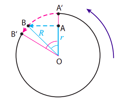
This is the angle shown in magenta in the figure. As a result of this rotation, the point A\(^{\prime}\) that was initially on the wall straight across from the puck has moved (following the magenta dashed line) to the position B\(^{\prime}\), so to an observer in the rotating room, looking at things from the point O, the puck appears to head for the wall and drift a little to the right while doing so.

The cyan angle in the picture, which we could call \(\Delta \theta_{part}\), has tangent equal to \(\sqrt{R^{2}-r^{2}} / r\), so we have

\[ \Delta \theta_{\text {room}}=\tan \left(\Delta \theta_{\text {part}}\right) \label{eq:8.64} .\]

This tells us the two angles are going to be pretty close if they are small enough, which is what happens if the puck starts close enough to the wall in the first place. The picture shows, for clarity, the case when \(r = 0.7R\), which gives \(\Delta \theta_{room}\) = 1.02 rad, and \(\Delta \theta_{part} = \tan^{−1}(1.02)\) = 0.8 rad. For \(r = 0.9R\), on the other hand, one finds \(\Delta \theta_{room}\) = 0.48 rad, and \(\Delta \theta_{part} = \tan^{−1}\)(0.48) = 0.45 rad.

In terms of pseudoforces (forces that do not, physically, exist, but may be introduced to describe mathematically the motion of objects in non-inertial frames of reference), the non-inertial observer would say that the puck heads towards the wall because of a centrifugal force (that is, a force pointing away from the center of rotation), and while doing so it drifts to the right because of the so-called Coriolis force.