
9.7: Induction, Transformers, and Generators


- Last updated
- Apr 10, 2025
- Save as PDF

( \newcommand{\kernel}{\mathrm{null}\,}\)
In this chapter we provide examples chosen to further familiarize you with Faraday’s Law of Induction and Lenz’s Law. The last example is the generator, the device used in the world’s power plants to convert mechanical energy into electrical energy.
A straight wire carries a current due northward. Due east of the straight wire, at the same elevation as the straight wire, is a horizontal loop of wire. The current in the straight wire is increasing. Which way is the current, induced in the loop by the changing magnetic field of the straight wire, directed around the loop? Solution
I’m going to draw the given situation from a few different viewpoints, just to help you get used to visualizing this kind of situation. As viewed from above-and-to-the-southeast, the configuration (aside from the fact that magnetic field lines are invisible) appears as:
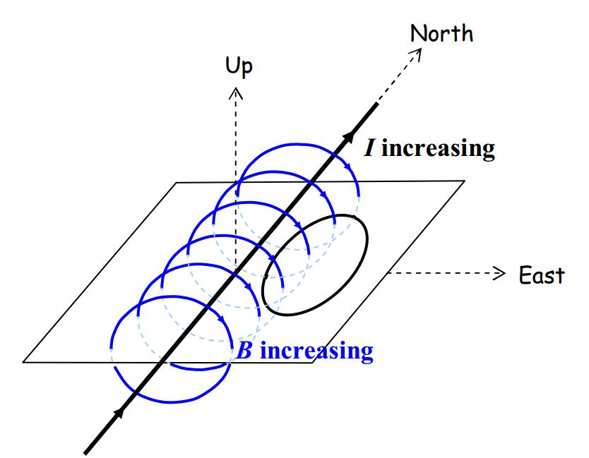
where I included a sheet of paper in the diagram to help you visualize things.
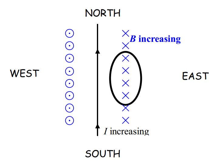
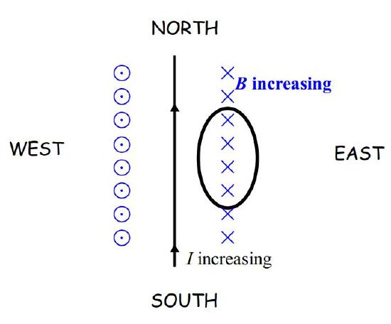
Here’s a view of the same configuration from the south, looking due north:
Both diagrams make it clear that we have an increasing number of downward-directed magnetic field lines through the loop. It is important to keep in mind that a field diagram is a diagrammatic manner of conveying information about an infinite set of vectors. There is no such thing as a curved vector. A vector is always directed along a straight line. The magnetic field vector is tangent to the magnetic field lines characterizing that vector. At the location of the loop, every magnetic field vector depicted in the diagram above is straight downward. While it is okay to say that we have an increasing number of magnetic field lines directed downward through the loop, please keep in mind that the field lines characterize vectors.
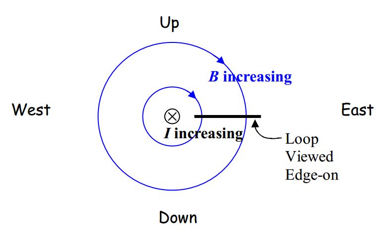
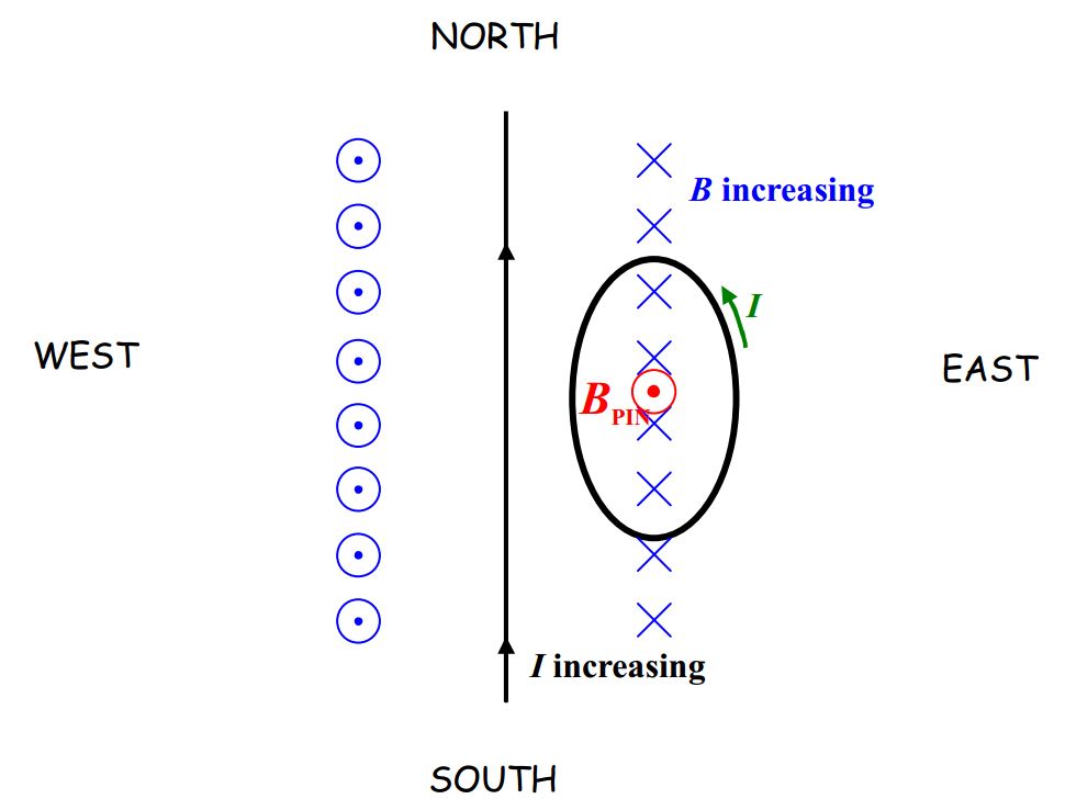
In presenting my solution to the example question, “What is the direction of the current induced in a horizontal loop that is due east of a straight wire carrying an increasing current due north?” I wouldn’t draw either one of the diagrams above. The first one takes too long to draw and there is no good way to show the direction of the current in the loop in the second one. The view from above is the most convenient one:
In this view (in which the downward direction is into the page) it is easy to see that what we have is an increasing number of downward-directed magnetic field lines through the loop (more specifically, through the region enclosed by the loop). In its futile attempt to keep the number of magnetic field lines directed downward through the loop the same as what it was, →BPIN must be directed upward in order to cancel out the newly-appearing downward-directed magnetic field lines. [Recall the sequence: The changing number of magnetic field lines induces (by Faraday’s Law) a current in the loop. That current produces (by Ampere’s Law) a magnetic field (→BPIN) of its own. Lenz’s Law relates the end product (→BPIN) to the original change (increasing number of downward-through-the-loop magnetic field lines).]
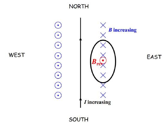
That’s interesting. We know the direction of the magnetic field produced by the induced current before we even known the direction of the induced current itself. So, what must the direction of the induced current be in order to produce an upward-directed magnetic field (→BPIN)? Well, by the right-hand rule for something curly something straight, the current must be counterclockwise, as viewed from above.
Solution
I’m going to draw the given situation from a few different viewpoints, just to help you get used to visualizing this kind of situation. As viewed from above-and-to-the-southeast, the configuration (aside from the fact that magnetic field lines are invisible) appears as:
where I included a sheet of paper in the diagram to help you visualize things.
Here’s a view of the same configuration from the south, looking due north:
Both diagrams make it clear that we have an increasing number of downward-directed magnetic field lines through the loop. It is important to keep in mind that a field diagram is a diagrammatic manner of conveying information about an infinite set of vectors. There is no such thing as a curved vector. A vector is always directed along a straight line. The magnetic field vector is tangent to the magnetic field lines characterizing that vector. At the location of the loop, every magnetic field vector depicted in the diagram above is straight downward. While it is okay to say that we have an increasing number of magnetic field lines directed downward through the loop, please keep in mind that the field lines characterize vectors.
In presenting my solution to the example question, “What is the direction of the current induced in a horizontal loop that is due east of a straight wire carrying an increasing current due north?” I wouldn’t draw either one of the diagrams above. The first one takes too long to draw and there is no good way to show the direction of the current in the loop in the second one. The view from above is the most convenient one:
In this view (in which the downward direction is into the page) it is easy to see that what we have is an increasing number of downward-directed magnetic field lines through the loop (more specifically, through the region enclosed by the loop). In its futile attempt to keep the number of magnetic field lines directed downward through the loop the same as what it was, →BPIN must be directed upward in order to cancel out the newly-appearing downward-directed magnetic field lines. [Recall the sequence: The changing number of magnetic field lines induces (by Faraday’s Law) a current in the loop. That current produces (by Ampere’s Law) a magnetic field (→BPIN) of its own. Lenz’s Law relates the end product (→BPIN) to the original change (increasing number of downward-through-the-loop magnetic field lines).]
That’s interesting. We know the direction of the magnetic field produced by the induced current before we even known the direction of the induced current itself. So, what must the direction of the induced current be in order to produce an upward-directed magnetic field (→BPIN)? Well, by the right-hand rule for something curly something straight, the current must be counterclockwise, as viewed from above.
Hey. That’s the answer to the question. We’re done with that example. Here’s another one:
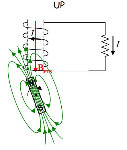
A person is moving a bar magnet, aligned north pole up, out from under a coil of wire, as
depicted below. What is the direction of the current in the resistor? 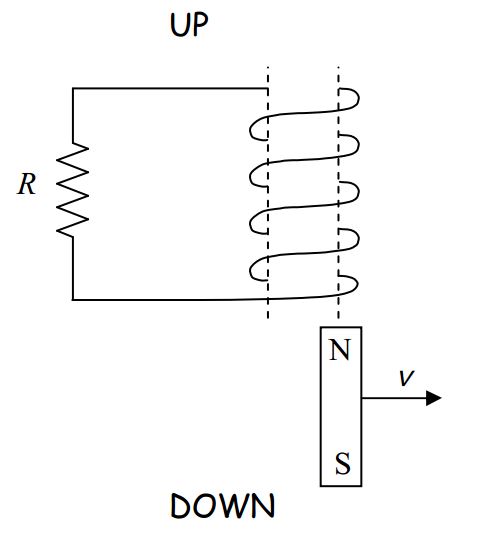
The magnetic field of the bar magnet extends upward through the coil.
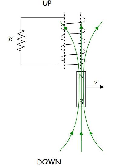
As the magnet moves out from under the coil, it takes its magnetic field with it. So, as regards the coil, what we have is a decreasing number of upward-directed magnetic field lines through the coil. By Faraday’s Law, this induces a current in the coil. By Ampere’s Law, the current produces a magnetic field, →BPIN. By Lenz’s Law →BPIN is upward, to make up for the departing upward-directed magnetic field lines through the coil.
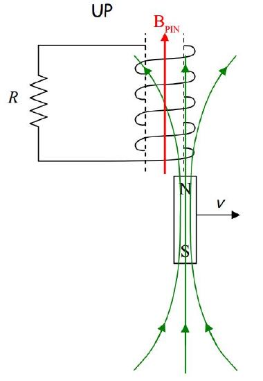
So, what is the direction of the current that is causing →BPIN? The right-hand rule will tell us that. Point the thumb of your cupped right hand in the direction of →BPIN. Your fingers will then be curled around (counterclockwise as viewed from above) in the direction of the current.
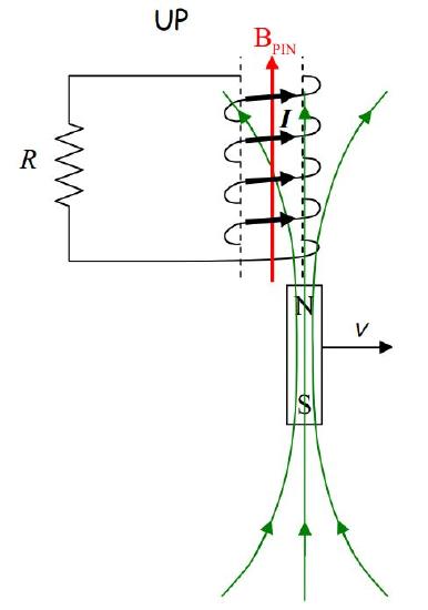
Because of the way the coil is wound, such a current will be directed out the top of the coil downward through the resistor.
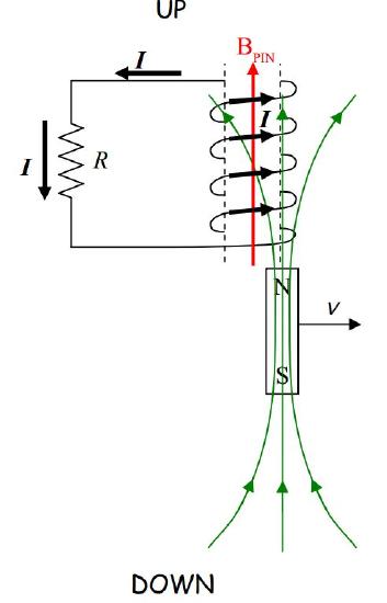
That’s the answer to the question posed in the example. (What is the direction of the current in the resistor?)
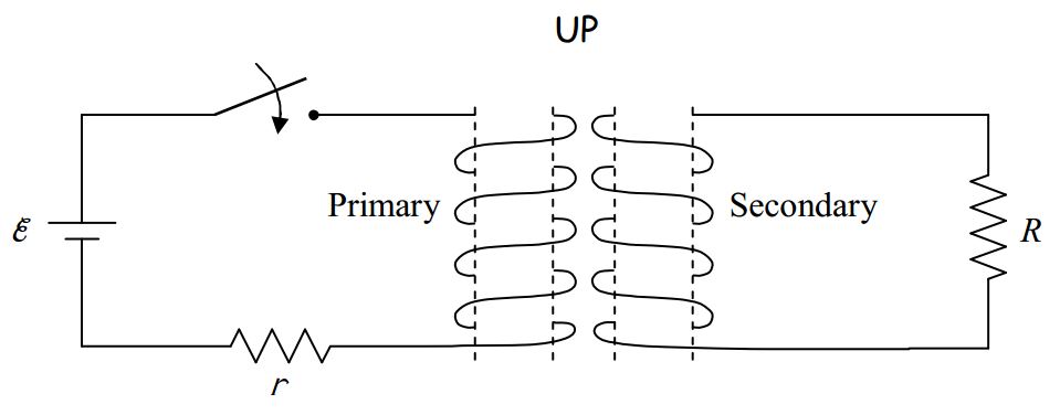
When you put two coils of wire near each other, such that when you create a magnetic field by using a seat of EMF to cause a current in one coil, that magnetic field extends through the region encircled by the other coil, you create a transformer. Let’s call the coil in which you initially cause the current, the primary coil, and the other one, the secondary coil. 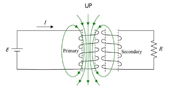
If you cause the current in the primary coil to be changing, then the magnetic field produced by that coil is changing. Thus, the flux through the secondary coil is changing, and, by Faraday’s Law of Induction, a current will be induced in the secondary coil. One way to cause the current in the primary coil to be changing would be to put a switch in the primary circuit (the circuit in which the primary coil is wired) and to repeatedly open and close it.
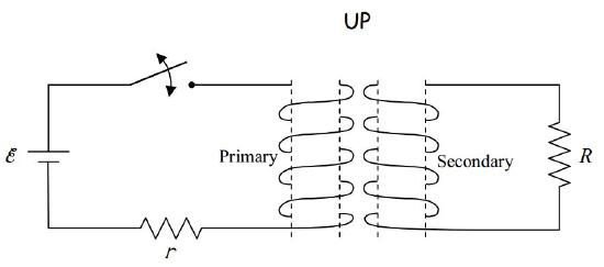
Okay, enough preamble, here’s the question: What is the direction of the transient current induced in the circuit above when the switch is closed?
Solution to Example 19-3:
Upon closing the switch, the current in the primary circuit very quickly builds up to ε/r. While the time that it takes for the current to build up to ε/r is very short, it is during this time interval that the current is changing. Hence, it is on this time interval that we must focus our attention in order to answer the question about the direction of the transient current in resistor R in the secondary circuit. The current in the primary causes a magnetic field. Because the current is increasing, the magnetic field vector at each point in space is increasing in magnitude.
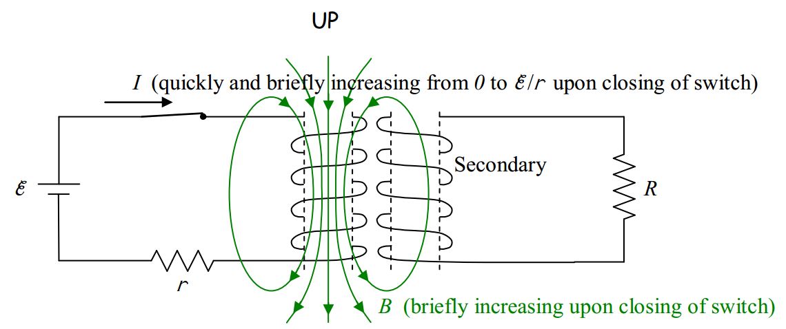
The increasing magnetic field causes upward-directed magnetic field lines in the region encircled by the secondary coil. There were no magnetic field lines through that coil before the switch was closed, so clearly, what we have here is an increasing number of upward-directed magnetic field lines through the secondary coil. By Faraday’s Law this will induce a current in the coil. By Ampere’s law, the current induced in the secondary will produce a magnetic field of its own, one that I like to call →BPIN for “The Magnetic field Produced by the Induced Current.” By Lenz’s Law, →BPIN must be downward to cancel out some of the newly-appearing upward-directed magnetic field lines through the secondary. (I hope it is clear that what I call the magnetic field lines through the secondary, are the magnetic field lines passing through the region encircled by the secondary coil.)
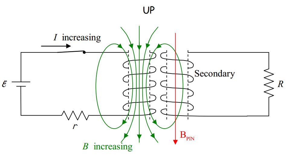
Okay. Now the question is, which way must the current be directed around the coil in order to create the downward-directed magnetic field →BPIN that we have deduced it does create. As usual, the right-hand rule for something curly something straight reveals the answer. We point the thumb of the cupped right hand in the direction of →BPIN and cannot fail to note that the fingers curl around in a direction that can best be described as “clockwise as viewed from above.”
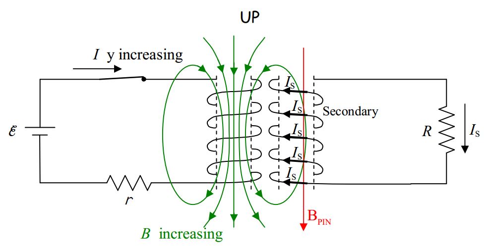
Because of the way the secondary coil is wound, such a current will be directed out of the secondary at the top of the coil and downward through resistor R. This is the answer to the
question posed in the example.
Solution to Example 19-3:
Upon closing the switch, the current in the primary circuit very quickly builds up to ε/r. While the time that it takes for the current to build up to ε/r is very short, it is during this time interval that the current is changing. Hence, it is on this time interval that we must focus our attention in order to answer the question about the direction of the transient current in resistor R in the secondary circuit. The current in the primary causes a magnetic field. Because the current is increasing, the magnetic field vector at each point in space is increasing in magnitude.
The increasing magnetic field causes upward-directed magnetic field lines in the region encircled by the secondary coil. There were no magnetic field lines through that coil before the switch was closed, so clearly, what we have here is an increasing number of upward-directed magnetic field lines through the secondary coil. By Faraday’s Law this will induce a current in the coil. By Ampere’s law, the current induced in the secondary will produce a magnetic field of its own, one that I like to call →BPIN for “The Magnetic field Produced by the Induced Current.” By Lenz’s Law, →BPIN must be downward to cancel out some of the newly-appearing upward-directed magnetic field lines through the secondary. (I hope it is clear that what I call the magnetic field lines through the secondary, are the magnetic field lines passing through the region encircled by the secondary coil.)
Okay. Now the question is, which way must the current be directed around the coil in order to create the downward-directed magnetic field →BPIN that we have deduced it does create. As usual, the right-hand rule for something curly something straight reveals the answer. We point the thumb of the cupped right hand in the direction of →BPIN and cannot fail to note that the fingers curl around in a direction that can best be described as “clockwise as viewed from above.”
Because of the way the secondary coil is wound, such a current will be directed out of the secondary at the top of the coil and downward through resistor R. This is the answer to the
question posed in the example.
An Electric Generator
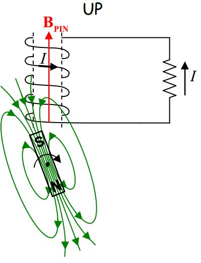
Consider a magnet that is caused to rotate in the vicinity of a coil of wire as depicted below.

As a result of the rotating magnet, the number and direction of the magnetic field lines through
the coil is continually changing. This induces a current in the coil, which, as it turns out, is also
changing. Check it out in the case of magnet that is, from our viewpoint, rotating clockwise. In
the orientation of the rotating magnet depicted here:

as the magnet rotates, the number of its magnetic field lines extending downward through the coil is decreasing. In accord with Faraday’s Law, this induces a current in the coil which, in accord with Ampere’s Law, produces a magnetic field of its own. By Lenz’s Law, the field (→BPIN) produced by the induced current must be downward to make up for the loss of downwarddirected magnetic field lines through the coil. To produce →BPIN downward, the induced current must be clockwise, as viewed from above. Based on the way the wire is wrapped and the coil is connected in the circuit, a current that is clockwise as viewed from above, in the coil, is directed out of the coil at the top of the coil and downward through the resistor.
In the following diagrams we show the magnet in each of several successive orientations. Keep in mind that someone or something is spinning the magnet by mechanical means. You can assume for instance that a person is turning the magnet with her hand. As the magnet turns the number of magnetic field lines is changing in a specific manner for each of the orientations depicted. You the reader are asked to apply Lenz’s Law and the Right Hand Rule for Something Curley, Something Straight to verify that the current (caused by the spinning magnet) through the resistor is in the direction depicted:

As the magnet continues to rotate clockwise, the next orientation it achieves is our starting point and the process repeats itself over and over again.
Recapping and extrapolating, the current through the resistor in the series of diagrams above, is:
downward, downward, upward, upward, downward, downward, upward, upward, …
For half of each rotation, the current is downward, and for the other half of each rotation, the current is upward. In quantifying this behavior, one focuses on the EMF induced in the coil:
The EMF across the coil varies sinusoidally with time as:
ε=εMAXsin(2πft)
where:
- ε which stands for EMF, is the time-varying electric potential difference between the terminals of a coil in close proximity to a magnet that is rotating relative to the coil as depicted in the diagrams above. This potential difference is caused to exist, and to vary the way it does, by the changing magnetic flux through the coil.
- εMAX is the maximum value of the EMF of the coil.
- f is the frequency of oscillations of the EMF across the coil. It is exactly equal to the rotation rate of the magnet expressed in rotations per second, a unit that is equivalent to hertz.

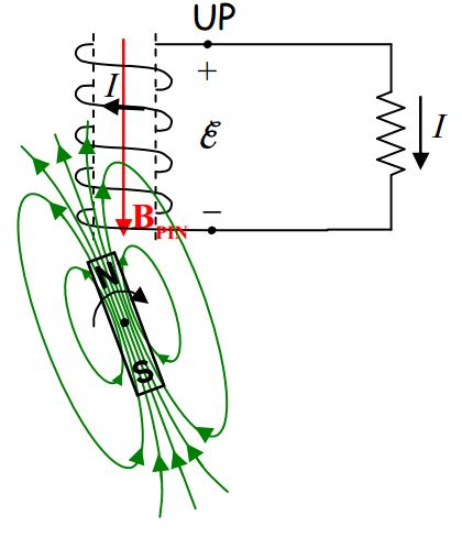
The device that we have been discussing (coil-plus-rotating magnet) is called a generator, or more specifically, an electric generator. A generator is a seat of EMF that causes there to be a potential difference between its terminals that varies sinusoidally with time. The schematic representation of such a time-varying seat of EMF is:

It takes work to spin the magnet. The magnetic field caused by the current induced in the coil exerts a torque on the magnet that always tends to slow it down. So, to keep the magnet spinning, one must continually exert a torque on the magnet in the direction in which it is spinning. The generator is the main component of any electrical power plant. It converts mechanical energy to electrical energy. The kind of power plant you are dealing with is determined by what your power company uses to spin the magnet. If moving water is used to spin the magnet, we call the power plant a hydroelectric plant. If a steam turbine is used to spin the magnet, then the power plant is designated by its method of heating and vaporizing water. For instance, if one heats and vaporizes the water by means of burning coal, one calls the power plant a coal-fired power plant. If one heats and vaporizes the water by means of a nuclear reactor, one calls the power plant a nuclear power plant.
Consider a “device which causes a potential difference between its terminals that varies sinusoidally with time” in a simple circuit:

The time-varying seat of EMF causes a potential difference across the resistor, in this simple circuit, equal, at any instant in time, to the voltage across the time-varying seat of EMF. As a result, there is a current in the resistor. The current is given by I=VR, our defining equation for resistance, solved for the current I. Because the algebraic sign of the potential difference across the resistor is continually alternating, the direction of the current in the resistor is continually alternating. Such a current is called an alternating current (AC). It has become traditional to use the abbreviation AC) to the extent that we do so in a redundant fashion, often referring to an alternating current as an AC current. (When we need to distinguish it from AC, we call the “oneway” kind of current that, say, a battery causes in a circuit, direct current, abbreviated DC.)
A device that causes current in a resistor, whether that current is alternating or not, is delivering energy to the resistor at a rate that we call power. The power delivered to a resistor can be expressed as P=IV where I is the current through the resistor and V is the voltage across the resistor. Using the defining equation of resistance, V=IR, the power can be expressed as P=I2R. A “device which causes a potential difference between its terminals that varies sinusoidally with time”, what I have been referring to as a “time-varying seat of EMF” is typically referred to as an AC power source. An AC power source is typically referred to in terms of the frequency of oscillations, and, the voltage that a DC power source, an ordinary seat of EMF, would have to maintain across its terminals to cause the same average power in any resistor that might be connected across the terminals of the AC power source. The voltage in question is typically referred to as εRMS or VRMS where the reasoning behind the name of the subscript will become evident shortly.
Since the power delivered by an ordinary seat of EMF is a constant, its average power is the value it always has.
Here’s the fictitious circuit
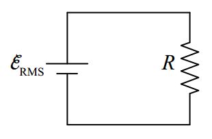
that would cause the same resistor power as the AC power source in question. The average power (which is just the power in the case of a DC circuit) is given by PAVG=IεRMS, which, by means of our defining equation of resistance solved for I, I=V/R, (where the voltage across the resistor is, by inspection, εRMS ) can be written PAVG=ε2RMSR. So far, this is old stuff, with an unexplained name for the EMF voltage. Now let’s consider the AC circuit:

The power is P=ε2R=[εMAXsin(2πft)]2R=ε2MAX[sin(2πft)]2R. The average value of the square of the sine function is 12. So the average power is PAVG=12ε2MAXR. Combining this with our expression PAVG=ε2RMSR from above yields:
ε2RMSR=12ε2MAXR
εRMS=√12εMAX
Now we are in a position to explain why we called the equivalent EMF, εRMS. In our expression PAVG=12ε2MAXR, we can consider ε2MAX2 to be the average value of the square of our timevarying EMF ε=εMAX=sin(2πft). Another name for “average” is “mean” so we can consider ε2MAX2 to be the mean value of ε2. On the right side of our expression for our equivalent EMF, εRMS=1√2εMAX, we have the square root of ε2MAX2, that is, we have the square root of the mean of the square of the EMF ε. And indeed the subscript “RMS” stands for “root mean squared.” RMS values are convenient for circuits consisting of resistors and AC power sources in that, one can analyze such circuits using RMS values the same way one analyzes DC circuits.
More on the Transformer
When the primary coil of a transformer is driven by an AC power source, it creates a magnetic field which varies sinusoidally in such a manner as to cause a sinusoidal EMF, of the same frequency as the source, to be induced in the secondary coil. The RMS value of the EMF induced in the secondary coil is directly proportional to the RMS value of the sinusoidal potential difference imposed across the primary. The constant of proportionality is the ratio of the number of turns in the secondary to the number of turns in the primary.
εSECONDARY=NSECONDARYNPRIMARYVPRIMARY
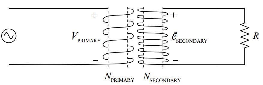
When the number of windings in the secondary coil is greater than the number of windings in the primary coil, the transformer is said to be a step-up transformer and the secondary voltage is greater than the primary voltage. When the number of windings in the secondary coil is less than the number of windings in the primary coil, the transformer is said to be a step-down transformer and the secondary voltage is less than the primary voltage.
The Electrical Power in Your House
When you plug your toaster into a wall outlet, you bring the prongs of the plug into contact with two conductors between which there is a time-varying potential difference characterized as 115 volts 60 Hz AC. The 60 Hz is the frequency of oscillations of the potential difference resulting from a magnet completing 60 rotations per second, back at the power plant. A step-up transformer is used near the power plant to step the power plant output up to a high voltage. Transmission lines at a very high potential, with respect to each other, provide a conducting path to a transformer near your home where the voltage is stepped down. Power lines at a much lower potential provide the conducting path to the wires in your home. 115 volts is the RMS value of the potential difference between the two conductors in each pair of slots in your wall outlets. Since εRMS=1√2εMAX, we have εMAX=√2 εRMS, so εMAX=√2(115volts), or εMAX=163volts. Thus,
ε=(163 volts)sin[2π(60Hz)t]
which can be written as,
ε=(163 volts)sin[(377radst]