2.12: The Electric Field (Answers)

Note: Answers are provided for only the odd-numbered questions.

Conceptual Questions

1. There are mostly equal numbers of positive and negative charges present, making the object electrically neutral.

3. a. yes; b. yes

5. Take an object with a known charge, either positive or negative, and bring it close to the rod. If the known charged object is positive and it is repelled from the rod, the rod is charged positive. If the positively charged object is attracted to the rod, the rod is negatively charged.

7. No, the dust is attracted to both because the dust particle molecules become polarized in the direction of the silk.

9. Yes, polarization charge is induced on the conductor so that the positive charge is nearest the charged rod, causing an attractive force.

11. Charging by conduction is charging by contact where charge is transferred to the object. Charging by induction first involves producing a polarization charge in the object and then connecting a wire to ground to allow some of the charge to leave the object, leaving the object charged.

13. This is so that any excess charge is transferred to the ground, keeping the gasoline receptacles neutral. If there is excess charge on the gasoline receptacle, a spark could ignite it.

15. The dryer charges the clothes. If they are damp, the presence of water molecules suppresses the charge.

17. There are only two types of charge, attractive and repulsive. If you bring a charged object near the quartz, only one of these two effects will happen, proving there is not a third kind of charge.

19. a. No, since a polarization charge is induced. b. Yes, since the polarization charge would produce only an attractive force.

21. The force holding the nucleus together must be greater than the electrostatic repulsive force on the protons.

23. Either sign of the test charge could be used, but the convention is to use a positive test charge.

25. The charges are of the same sign.

27. At infinity, we would expect the field to go to zero, but because the sheet is infinite in extent, this is not the case. Everywhere you are, you see an infinite plane in all directions.

29. The infinite charged plate would have \(\displaystyle E=\frac{σ}{2ε_0}\) everywhere. The field would point toward the plate if it were negatively charged and point away from the plate if it were positively charged. The electric field of the parallel plates would be zero between them if they had the same charge, and E would be \(\displaystyle E=\frac{σ}{ε_0}\) everywhere else. If the charges were opposite, the situation is reversed, zero outside the plates and \(\displaystyle E=\frac{σ}{ε_0}\) between them.

31. yes; no

33. At the surface of Earth, the gravitational field is always directed in toward Earth’s center. An electric field could move a charged particle in a different direction than toward the center of Earth. This would indicate an electric field is present.

35. 10

Problems

37. a. \(\displaystyle 2.00×10^{−9}C(\frac{1}{1.602×10^{−19}}e/C)=1.248×10^{10}electrons2\);

b. \(\displaystyle 0.500×10^{−6}C(\frac{1}{1.602×10^{−19}}e/C)=3.121×10^{12}electrons\)

39. \(\displaystyle \frac{3.750×10^{21}e}{6.242×10^{18}e/C}=-600.8C\)

41. a. \(2.0×10^{−9}C(6.242×10^{18}e/C)=1.248×10^{10}e\);

b. \(\displaystyle 9.109×10^{−31}kg(1.248×10^{10}e)=1.137×10^{−20}kg, \frac{1.137×10^{−20}kg}{2.5×10^{−3}kg}=4.548×10^{−18}\) or \(\displaystyle 4.545×10^{−16}%\)

43. \(\displaystyle 5.00×10^{−9}C(6.242×10^{18}e/C)=3.121×10^{10}e; 3.121×10^{10}e+1.0000×10^{12}e=1.0312×10^{12}e\).

45. atomic mass of copper atom times \(\displaystyle 1u=1.055×10^{−25}kg\); number of copper atoms = \(\displaystyle 4.739×10^{23}atoms\); number of electrons equals 29 times number of atoms or \(\displaystyle 1.374×10^{25}electrons\); \(\displaystyle \frac{2.00×10^{−6}C(6.242×10^{18}e/C)}{1.374×10^{25}e}=9.083×10^{−13}\) or \(\displaystyle 9.083×10^{−11}%\).

47. \(\displaystyle 244.00u(1.66×10^{−27}kg/u)=4.050×10^{−25}kg\); \(\displaystyle \frac{4.00kg}{4.050×10^{−25}kg}=9.877×10^{24}atoms\) \(\displaystyle 9.877×10^{24}(94)=9.284×10^{26}protons\) \(\displaystyle 9.284×10^{26}protons; 9.284×10^{26}(1.602×10^{−19}C/p)=1.487×10^8C\)

49. a. charge 1 is \(\displaystyle 3μC\); charge 2 is \(\displaystyle 12μC\), \(\displaystyle F_{31}=2.16×10^{−4}N\) to the left,

\(\displaystyle F_{32}=8.63×10^{−4}N\) to the right,

\(\displaystyle F_{net}=6.47×10^{−4}N\) to the right;

b. \(\displaystyle F_{31}=2.16×10^{−4}N\) to the right,

\(\displaystyle F_{32}=9.59×10^{−5}N\) to the right,

\(\displaystyle F_{net}=3.12×10^{−4}N\) to the right,

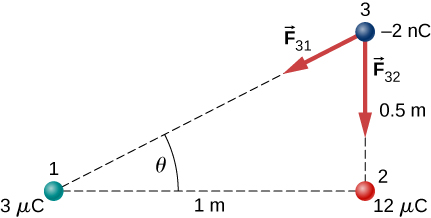
c. \(\displaystyle \vec{F}_{31x}=−2.76×10^{−5}N\hat{i},\)

\(\displaystyle \vec{F}_{31y}=−1.38×10^{−5}N\hat{j}\),

\(\displaystyle \vec{F}_{32y}=−8.63×10^{−4}N\hat{j}\),

\(\displaystyle \vec{F}_{net}=−2.76×10^{−5}N\hat{i}−8.77×10^{−4}N\hat{j}\)

51. \(\displaystyle F=230.7N\)

53. \(\displaystyle F=53.94N\)

55. The tension is \(\displaystyle T=0.049N\). The horizontal component of the tension is \(\displaystyle 0.0043N\)

\(\displaystyle d=0.088m,q=6.1×10^{−8}C\).

The charges can be positive or negative, but both have to be the same sign.

57. Let the charge on one of the spheres be rQ, where r is a fraction between 0 and 1. In the numerator of Coulomb’s law, the term involving the charges is \(\displaystyle rQ(1−r)Q\). This is equal to \(\displaystyle (r−r^2)Q^2\). Finding the maximum of this term gives \(\displaystyle 1−2r=0⇒r=\frac{1}{2}\)

59. Define right to be the positive direction and hence left is the negative direction, then \(\displaystyle F=−0.05N\)

61. The particles form triangle of sides 13, 13, and 24 cm. The x-components cancel, whereas there is a contribution to the y-component from both charges 24 cm apart. The y-axis passing through the third charge bisects the 24-cm line, creating two right triangles of sides 5, 12, and 13 cm. \(\displaystyle F_y=2.56N\) in the negative y-direction since the force is attractive. The net force from both charges is \(\displaystyle \vec{F}_{net}=−5.12N\hat{j}\)

63. The diagonal is \(\displaystyle \sqrt{2}a\) and the components of the force due to the diagonal charge has a factor \(\displaystyle cosθ=\frac{1}{\sqrt{2}}\); \(\displaystyle \vec{F}_{net}=[k\frac{q^2}{a^2}+k\frac{q^2}{2a^2}\frac{1}{\sqrt{2}}]\hat{i}−[k\frac{q^2}{a^2}+k\frac{q^2}{2a^2}\frac{1}{\sqrt{2}}]\hat{j}\)

65. \(\displaystyle a. E=2.0×10^{−2}\frac{N}{C}\);

\(\displaystyle b. F=2.0×10^{−19}N\)

67. a. \(\displaystyle E=2.88×10^{11}N/C\);

b. \(\displaystyle E=1.44×10^{11}N/C\);

c. \(\displaystyle F=4.61×10^{−8}N\) on alpha particl

\(\displaystyle F=4.61×10^{−8}N\) on electron

69. \(\displaystyle E=(−2.0\hat{i}+3.0\hat{j})N\)

71. \(\displaystyle F=3.204×10^{−14}N\),

\(\displaystyle a=3.517×10^{16}m/s^2\)

73. \(\displaystyle q=2.78×10^{−9}C\)

75. a. \(\displaystyle E=1.15×10^{12}N/C\);

b. \(\displaystyle F=1.47×10^{−6}N\)

77. If the \(\displaystyle q_2\) is to the right of \(\displaystyle q_1\), the electric field vector from both charges point to the right.

a. \(\displaystyle E=2.70×10^6N/C\);

b. \(\displaystyle F=54.0N\)

79. There is 45° right triangle geometry. The x-components of the electric field at \(\displaystyle y=3m\) cancel. The y-components give \(\displaystyle E(y=3m)=2.83×10^3N/C\).

At the origin we have a a negative charge of magnitide \(\displaystyle q=−2.83×10^{−6}C\)

81. \(\displaystyle \vec{E}(z)=3.6×10^4N\hat{k}\)

85. \(\displaystyle σ=0.02C/m^2\) \(\displaystyle E=2.26×10^9N/C\)

89. a. \(\displaystyle \vec{E}(\vec{r})=\frac{1}{4πε_0}\frac{2λ_x}{a}\hat{i}+\frac{1}{4πε_0}\frac{2λ_y}{b}\hat{j}\);

b. \(\displaystyle \frac{1}{4πε_0}\frac{2(λ_x+λ_y)}{c}\hat{k}\)

91. a. \(\displaystyle \vec{F}=3.2×10^{−17}N\hat{i}\),

\(\displaystyle \vec{a}=1.92×10^{10}m/s^2\hat{i}\);

b. \(\displaystyle \vec{F} =−3.2×10^{−17}N\hat{i}\),

\(\displaystyle \vec{a} =−3.51×10^{13}m/s^2\hat{i}\)

93. \(\displaystyle m=6.5×10^{−11}kg\),

\(\displaystyle E=1.6×10^7N/C\)

95. \(\displaystyle E=1.70×10^6N/C\),

\(\displaystyle F=1.53×10^{−3}NTcosθ=mgTsinθ=qE\),

\(\displaystyle tanθ=0.62⇒θ=32.0°\),

This is independent of the length of the string.

99. a. \(\displaystyle W=\frac{1}{2}m(v^2−v^2_0), \frac{Qq}{4πε_0}(\frac{1}{r}−\frac{1}{r_0})=\frac{1}{2}m(v^2−v^2_0)⇒r_0−r=\frac{4πε_0}{Qq}\frac{1}{2}rr_0m(v^2−v^2_0)\);

b. \(\displaystyle r_0−r\) is negative; therefore, \(\displaystyle v_0>v, r→∞\), and \(\displaystyle v→0:\frac{Qq}{4πε_0}(−\frac{1}{r_0})=−\frac{1}{2}mv^2_0⇒v_0=\sqrt{\frac{Qq}{2πε_0mr_0}}\)

101.

103.

Additional Problems

109. \(\displaystyle \vec{F}_{net}=[−8.99×10^9\frac{3.0×10^{−6}(5.0×10^{−6})}{(3.0m)^2}−8.99×10^9\frac{9.0×10^{−6}(5.0×10^{−6})}{(3.0m)^2}]\hat{i}, −8.99×10^9\frac{6.0×10^{−6}(5.0×10^{−6})}{(3.0m)^2}\hat{j}=−0.06N\hat{i}−0.03N\hat{j}\)

111. Charges Q and q form a right triangle of sides 1 m and \(\displaystyle 3+\sqrt{3}m.\) Charges 2Q and q form a right triangle of sides 1 m and \(\displaystyle \sqrt{3}m\).

\(\displaystyle F_x=0.049N,\)

\(\displaystyle F_y=0.09N\),

\(\displaystyle \vec{F}_{net}=0.049N\hat{i}+0.09N\hat{j}\)

113. W=0.054J

115. a. \(\displaystyle \vec{E}=\frac{1}{4πε_0}(\frac{q}{(2a)^2}−\frac{q}{a^2})\hat{i}\);

b. \(\displaystyle \vec{E}=\frac{\sqrt{3}}{4πε_0}\frac{q}{a^2}(−\hat{j})\);

c. \(\displaystyle \vec{E}=\frac{2}{πε_0}\frac{q}{a^2}\frac{1}{\sqrt{2}}(−\hat{j})\)

117. \(\displaystyle \vec{E}=6.4×10^6(\hat{i})+1.5×10^7(\hat{j})N/C\)

119. \(\displaystyle F=qE_0(1+x/a)\) \(\displaystyle W=\frac{1}{2}m(v^2−v^2_0)\),

\(\displaystyle \frac{1}{2}mv^2=qE_0(\frac{15a}{2})J\)

Contributors and Attributions

Samuel J. Ling (Truman State University), Jeff Sanny (Loyola Marymount University), and Bill Moebs with many contributing authors. This work is licensed by OpenStax University Physics under a Creative Commons Attribution License (by 4.0).