4.1: Electric Potential from Electric Field

Learning Objectives

By the end of this section, you will be able to:

• Calculate electric potential change from the electric field in a region of space.
• Relate the voltage drop across charged parallel plates to their intervening electric field.

So far, we have explored the relationship between voltage and energy. Now we want to explore the relationship between voltage and electric field. We will start with the general case for a non-uniform \(\vec{E}\) field. Recall that our general formula for the potential energy of a test charge \(q\) at point \(P\) relative to reference point \(R\) is

\[U_p = - \int_R^P \vec{F} \cdot d\vec{l}.\]

When we substitute in the definition of electric field \((\vec{E} = \vec{F}/q)\), this becomes

\[U_p = -q \int_R^P \vec{E} \cdot d\vec{l}.\]

Applying our definition of potential \((V = U/q)\) to this potential energy, we find that, in general,

\[V_p = - \int_R^P \vec{E} \cdot d\vec{l}. \label{PotentialandField}\]

From our previous discussion of the potential energy of a charge in an electric field, the result is independent of the path chosen, and hence we can pick the integral path that is most convenient.

Consider the special case of a positive point charge \(q\) at the origin. To calculate the potential caused by \(q\) at a distance \(r\) from the origin relative to a reference of 0 at infinity (recall that we did the same for potential energy), let \(P = r\) and \(R = \infty\), with \(d\vec{l} = d\vec{r} = \hat{r}dr\) and use \(\vec{E} = \frac{kq}{r^2} \hat{r}\). When we evaluate the integral

\[V_p = - \int_R^P \vec{E} \cdot d\vec{l}\] for this system, we have

\[V_r = - \int_{\infty}^r \dfrac{kq}{r^2} dr = \dfrac{kq}{r} - \dfrac{kq}{\infty} = \dfrac{kq}{r}.\]

This result,

\[V_r = \dfrac{kq}{r}\]

is the standard form of the potential of a point charge. This will be explored further in the next section.

To examine another interesting special case, suppose a uniform electric field \(\vec{E}\) is produced by placing a potential difference (or voltage) \(\Delta V\) across two parallel metal plates, labeled \(A\) and \(B\) (Figure \(\PageIndex{1}\)). Examining this situation will tell us what voltage is needed to produce a certain electric field strength. It will also reveal a more fundamental relationship between electric potential and electric field.

Figure \(\PageIndex{1}\): The relationship between \(V\) and \(E\) for parallel conducting plates is \(E = V/d\). (Note that \(\Delta V = V_{AB}\) in magnitude. For a charge that is moved from plate \(A\) at higher potential to plate \(B\) at lower potential, a minus sign needs to be included as follows: \(- \Delta V = V_A - V_B = V_{AB}\).)

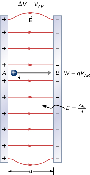
From a physicist’s point of view, either \(\Delta V\) or \(\vec{E}\) can be used to describe any interaction between charges. However, \(\Delta V\) is a scalar quantity and has no direction, whereas \(\vec{E}\) is a vector quantity, having both magnitude and direction. (Note that the magnitude of the electric field, a scalar quantity, is represented by \(E\).) The relationship between \(\Delta V\) and \(\vec{E}\) is revealed by calculating the work done by the electric force in moving a charge from point \(A\) to point \(B\). But, as noted earlier, arbitrary charge distributions require calculus. We therefore look at a uniform electric field as an interesting special case.

The work done by the electric field in Figure \(\PageIndex{1}\) to move a positive charge \(q\) from \(A\), the positive plate, higher potential, to \(B\), the negative plate, lower potential, is

\[W = - \Delta U = - q\Delta V.\]

The potential difference between points \(A\) and \(B\) is

\[- \Delta V = - (V_B - V_A) = V_A - V_B = V_{AB}.\]

Entering this into the expression for work yields

\[W = qV_{AB}.\]

Work is \(W = \vec{F} \cdot \vec{d} = Fd \, \cos\theta\): here \(\cos \theta = 1\), since the path is parallel to the field. Thus, \(W = Fd\). Since \(F = qE\) we see that \(W = qEd\).

Substituting this expression for work into the previous equation gives

\[qEd = qV_{AB}.\]

The charge cancels, so we obtain for the voltage between points \(A\) and \(B\)

\[
\left.
\begin{array}{c}
V_{AB} = Ed \\
E = \dfrac{V_{AB}}{d}
\end{array}
\right\}
\ \textrm{(uniform}\ E\textrm{-field only)}
\]

where \(d\) is the distance from \(A\) to \(B\), or the distance between the plates in Figure \(\PageIndex{1}\). Note that this equation implies that the units for electric field are volts per meter. We already know the units for electric field are newtons per coulomb; thus, the following relation among units is valid:

\[1 \, \textrm{N/C} = 1 \, \textrm{V/m}.\]

Furthermore, we may extend this to the integral form. Substituting Equation \ref{PotentialandField} into our definition for the potential difference between points \(A\) and \(B\), we obtain

\[V_{AB} = V_B - V_A = - \int_R^B \vec{E} \cdot d\vec{l} + \int_R^A \vec{E} \cdot d\vec{l}\]

which simplifies to

\[V_B - V_A = - \int_A^B \vec{E} \cdot d\vec{l}.\]

As a demonstration, from this we may calculate the potential difference between two points (\(A\) and \(B\)) equidistant from a point charge \(q\) at the origin, as shown in Figure \(\PageIndex{2}\).

Figure \(\PageIndex{2}\): The arc for calculating the potential difference between two points that are equidistant from a point charge at the origin.

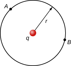
To do this, we integrate around an arc of the circle of constant radius r between \(A\) and \(B\), which means we let \(d\vec{l} = r\hat{\varphi}d\varphi\), while using \(\vec{E} = \frac{kq}{r^2} \hat{r}\). Thus,

\[\Delta V = V_B - V_A = - \int_A^B \vec{E} \cdot d\vec{l}.\]

for this system becomes

\[V_B - V_A = - \int_A^B \frac{kq}{r^2} \hat{r} \cdot r\hat{\varphi}d\varphi.\]

However, \(\hat{r} \cdot \hat{\varphi}\) and therefore

\[V_B - V_A = 0.\]

This result, that there is no difference in potential along a constant radius from a point charge, will come in handy when we map potentials.

Example \(\PageIndex{1A}\): What Is the Highest Voltage Possible between Two Plates?

Dry air can support a maximum electric field strength of about \(3.0 \times 10^6 \textrm{V/m}\). Above that value, the field creates enough ionization in the air to make the air a conductor. This allows a discharge or spark that reduces the field. What, then, is the maximum voltage between two parallel conducting plates separated by 2.5 cm of dry air?

Strategy

We are given the maximum electric field \(E\) between the plates and the distance \(d\) between them. We can use the equation \(V_{AB} = Ed\) to calculate the maximum voltage.

Solution

The potential difference or voltage between the plates is

\[V_{AB} = Ed.\]

Entering the given values for \(E\) and \(d\) gives

\[V_{AB} = (3.0 \times 10^6 \textrm{V/m})(0.025 \, \textrm{m}) = 7.5 \times 10^4 \, \textrm{V}\] or \[V_{AB} = 75 \, \textrm{kV}.\]

(The answer is quoted to only two digits, since the maximum field strength is approximate.)

Significance

One of the implications of this result is that it takes about 75 kV to make a spark jump across a 2.5-cm (1-in.) gap, or 150 kV for a 5-cm spark. This limits the voltages that can exist between conductors, perhaps on a power transmission line. A smaller voltage can cause a spark if there are spines on the surface, since sharp points have larger field strengths than smooth surfaces. Humid air breaks down at a lower field strength, meaning that a smaller voltage will make a spark jump through humid air. The largest voltages can be built up with static electricity on dry days (Figure \(\PageIndex{3}\)).

Figure \(\PageIndex{3}\): A spark chamber is used to trace the paths of high-energy particles. Ionization created by the particles as they pass through the gas between the plates allows a spark to jump. The sparks are perpendicular to the plates, following electric field lines between them. The potential difference between adjacent plates is not high enough to cause sparks without the ionization produced by particles from accelerator experiments (or cosmic rays). This form of detector is now archaic and no longer in use except for demonstration purposes. (credit b: modification of work by Jack Collins)

Example \(\PageIndex{1B}\): Field and Force inside an Electron Gun

An electron gun has parallel plates separated by 4.00 cm and gives electrons 25.0 keV of energy. (a) What is the electric field strength between the plates? (b) What force would this field exert on a piece of plastic with a \(0.500-\mu \textrm{C}\) charge that gets between the plates?

Strategy

Since the voltage and plate separation are given, the electric field strength can be calculated directly from the expression \(E = \frac{V_{AB}}{d}\). Once we know the electric field strength, we can find the force on a charge by using \(\vec{F} = q\vec{E}\). Since the electric field is in only one direction, we can write this equation in terms of the magnitudes, \(F = qE\).

Solution

a. The expression for the magnitude of the electric field between two uniform metal plates is

\[E = \dfrac{V_{AB}}{d}.\] Since the electron is a single charge and is given 25.0 keV of energy, the potential difference must be 25.0 kV. Entering this value for \(V_{AB}\) and the plate separation of 0.0400 m, we obtain \[E = \frac{25.0 \, \textrm{kV}}{0.0400 \, \textrm{m}} = 6.25 \times 10^5 \, \textrm{V/m}.\]

b. The magnitude of the force on a charge in an electric field is obtained from the equation \[F = qE.\] Substituting known values gives

\[F = (0.500 \times 10^{-6}\textrm{C})(6.25 \times 10^5 \textrm{V/m}) = 0.313 \, \textrm{N}.\]

Significance

Note that the units are newtons, since \(1 \, \textrm{V/m} = 1 \, \textrm{N/C}\). Because the electric field is uniform between the plates, the force on the charge is the same no matter where the charge is located between the plates.

Example \(\PageIndex{1C}\): Calculating Potential of a Point Charge

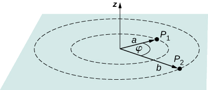
Given a point charge \(q = +2.0 \textrm{nC}\) at the origin, calculate the potential difference between point \(P_1\) a distance \(a = 4.0 \, \textrm{cm}\) from \(q\), and \(P_2\) a distance \(b = 12.0 \, \textrm{cm}\) from \(q\), where the two points have an angle of \(\varphi = 24^\circ\) between them (Figure \(\PageIndex{4}\)).

Figure \(\PageIndex{4}\): Find the difference in potential between \(P_1\) and \(P_2\).

Strategy

Do this in two steps. The first step is to use \(V_B - V_A = -\int_A^B \vec{E} \cdot d\vec{l}\) and let \(A = a = 4.0 \, cm\) and \(B = b = 12.0 \, \textrm{cm}\), with \(d\vec{l} = d\vec{r} = \hat{r}dr\) and \(\vec{E} = \frac{kq}{r^2} \hat{r}.\) Then perform the integral. The second step is to integrate \(V_B - V_A = -\int_A^B \vec{E} \cdot d\vec{l}\) around an arc of constant radius \(r\), which means we let \(d\vec{l} = r\vec{\varphi}d\varphi\) with limits \(0 \leq \varphi \leq 24^\circ\), still using \(\vec{E} = \frac{kq}{r^2}\hat{r}\).

Then add the two results together.

Solution

For the first part, \(V_B - V_A = -\int_A^B \vec{E} \cdot d\vec{l}\) for this system becomes \(V_b - V_a = - \int_a^b \frac{kq}{r^2}\hat{r} \cdot \hat{r}dr\) which computes to

\(\Delta V = - \int_a^b \frac{kq}{r^2}dr = kq \left[\frac{1}{a} - \frac{1}{b}\right]\)

\(= (8.99 \times 10^9 \textrm{N}\cdot\textrm{m}^2/\textrm{C}^2)(2.0 \times 10^{-9}\textrm{C}) \left[\frac{1}{0.040 \, \textrm{m}} - \frac{1}{0.12 \, \textrm{m}}\right] = 300 \, \textrm{V}\).

For the second step, \(V_B - V_A = -\int_A^B \vec{E} \cdot d\vec{l}\) becomes \(\Delta V = - \int_{0}^{24\pi/180} \frac{kq}{r^2} \hat{r} \cdot r\hat{\varphi}d\varphi\), but \(\hat{r} \cdot \hat{\varphi} = 0\) and therefore \(\Delta V = 0\). Adding the two parts together, we get 300 V.

Significance

We have demonstrated the use of the integral form of the potential difference to obtain a numerical result. Notice that, in this particular system, we could have also used the formula for the potential due to a point charge at the two points and simply taken the difference.

Exercise \(\PageIndex{4}\)

From the examples, how does the energy of a lightning strike vary with the height of the clouds from the ground? Consider the cloud-ground system to be two parallel plates.

Answer

Given a fixed maximum electric field strength, the potential at which a strike occurs increases with increasing height above the ground. Hence, each electron will carry more energy. Determining if there is an effect on the total number of electrons lies in the future.